【CNN网络入门】基于PyTorch的MNIST手写数字识别：从数据准备到模型部署全流程详解

前言

手写数字识别是计算机视觉领域的经典入门项目，MNIST数据集包含了大量0-9的手写数字图片，是深度学习入门的"Hello World"。本文将详细介绍如何使用PyTorch框架构建一个卷积神经网络（CNN）来识别MNIST手写数字，并展示完整的训练、评估和可视化流程。

实验环境

操作系统: Windows/Linux/MacOS
Python版本: 3.7±
深度学习框架: PyTorch 1.8+
其他库: torchvision, matplotlib, numpy
硬件: 支持GPU加速（可选）

一、数据准备与预处理

1.1 设置GPU加速

在深度学习中，GPU可以显著加速模型训练。我们首先检查并设置计算设备：

python 复制代码

import torch
import torch.nn as nn
import matplotlib.pyplot as plt
import torchvision

# 设置硬件设备，优先使用GPU
device = torch.device("cuda" if torch.cuda.is_available() else "cpu")
print(f"当前使用设备: {device}")

device(type='cpu')

1.2 加载MNIST数据集

PyTorch的torchvision模块提供了方便的MNIST数据加载功能：

python 复制代码

# 加载训练集和测试集
train_ds = torchvision.datasets.MNIST('data', 
                                      train=True, 
                                      transform=torchvision.transforms.ToTensor(),
                                      download=True)

test_ds = torchvision.datasets.MNIST('data', 
                                     train=False, 
                                     transform=torchvision.transforms.ToTensor(),
                                     download=True)

参数说明：

train=True/False: 指定加载训练集还是测试集
transform=torchvision.transforms.ToTensor(): 将PIL图像转换为Tensor格式
download=True: 如果本地没有数据集则自动下载

1.3 创建数据加载器

数据加载器（DataLoader）可以批量加载数据，支持数据打乱和并行加载：

python 复制代码

batch_size = 32

train_dl = torch.utils.data.DataLoader(train_ds, 
                                       batch_size=batch_size, 
                                       shuffle=True)

test_dl = torch.utils.data.DataLoader(test_ds, 
                                       batch_size=batch_size)

二、数据可视化

在开始训练前，我们先查看一下数据的样子：

python 复制代码

import numpy as np

# 获取一个批次的训练数据
imgs, labels = next(iter(train_dl))
print(f"数据形状: {imgs.shape}")  # [batch_size, channel, height, width]

# 可视化前20张图片
plt.figure(figsize=(20, 5))
for i, img in enumerate(imgs[:20]):
    # 去除通道维度（从[1,28,28]变为[28,28]）
    npimg = np.squeeze(img.numpy())
    
    # 创建子图
    plt.subplot(2, 10, i+1)
    plt.imshow(npimg, cmap=plt.cm.binary)
    plt.title(f"Label: {labels[i].item()}")
    plt.axis('off')

plt.show()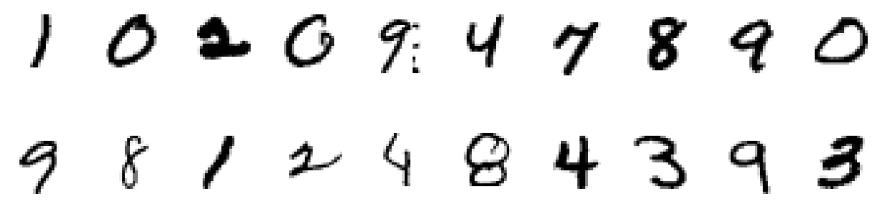

从图中可以看出，MNIST数据集中的图片是28×28像素的灰度图像，每个图像对应一个0-9的数字标签。

三、构建卷积神经网络（CNN）

3.1 CNN网络结构设计

我们设计一个包含两个卷积层和两个全连接层的简单CNN网络：

python 复制代码

import torch.nn.functional as F

num_classes = 10  # 输出类别数（0-9）

class Model(nn.Module):
    def __init__(self):
        super().__init__()
        # 特征提取网络
        self.conv1 = nn.Conv2d(1, 32, kernel_size=3)  # 输入通道1，输出通道32
        self.pool1 = nn.MaxPool2d(2)                  # 2×2最大池化
        self.conv2 = nn.Conv2d(32, 64, kernel_size=3) # 输入通道32，输出通道64
        self.pool2 = nn.MaxPool2d(2)
        
        # 分类网络
        self.fc1 = nn.Linear(1600, 64)          # 全连接层1
        self.fc2 = nn.Linear(64, num_classes)   # 全连接层2（输出层）
    
    def forward(self, x):
        # 卷积层1 + ReLU激活 + 池化层1
        x = self.pool1(F.relu(self.conv1(x)))
        
        # 卷积层2 + ReLU激活 + 池化层2
        x = self.pool2(F.relu(self.conv2(x)))
        
        # 展平特征图
        x = torch.flatten(x, start_dim=1)
        
        # 全连接层
        x = F.relu(self.fc1(x))
        x = self.fc2(x)
        
        return x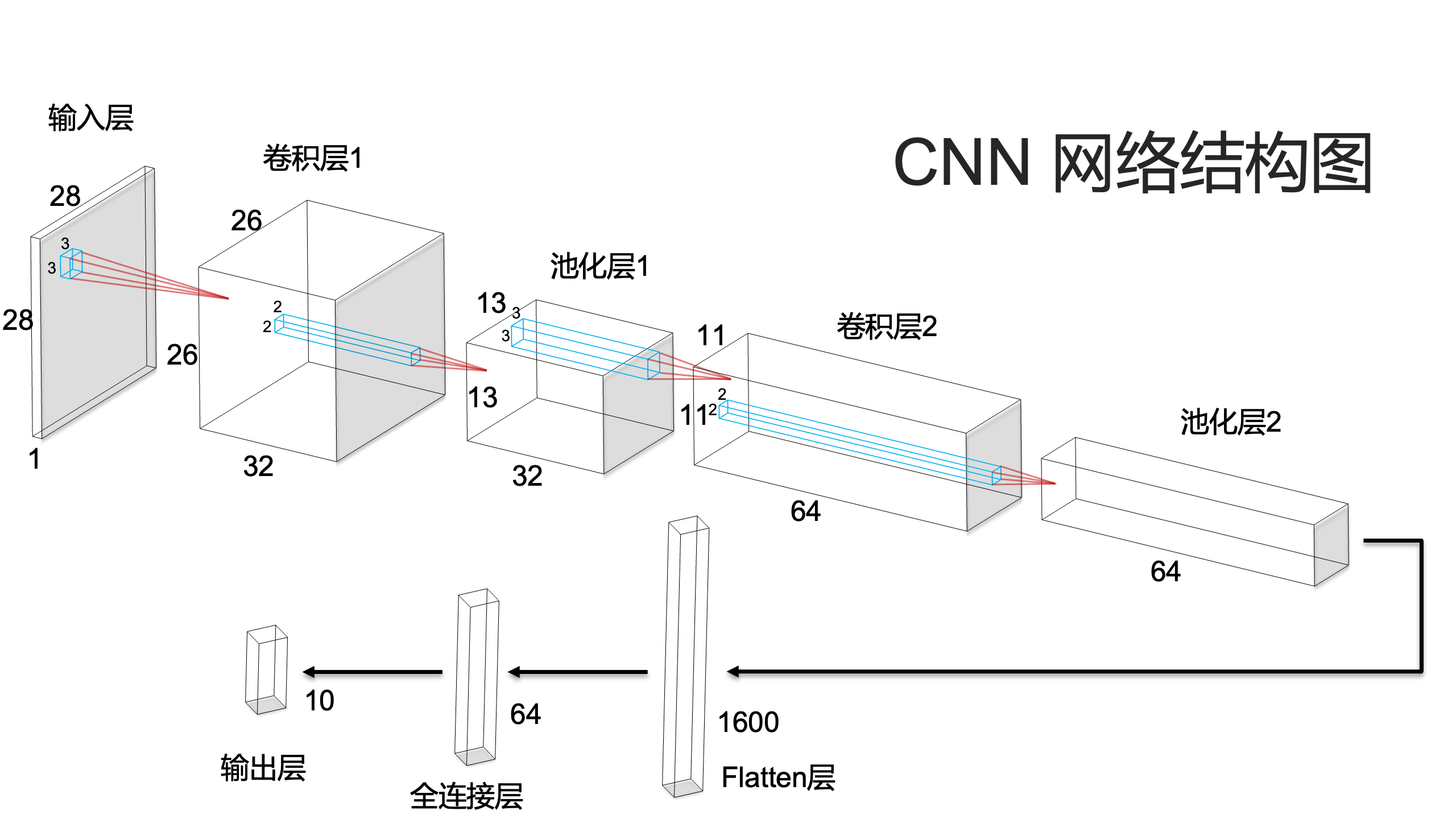

3.2 网络结构分析

使用torchinfo库查看网络详细结构：

python 复制代码

from torchinfo import summary

model = Model().to(device)
summary(model)

输出结果：

复制代码

=================================================================
Layer (type:depth-idx)                   Param #
=================================================================
Model                                    --
├─Conv2d: 1-1                            320
├─MaxPool2d: 1-2                         --
├─Conv2d: 1-3                            18,496
├─MaxPool2d: 1-4                         --
├─Linear: 1-5                            102,464
├─Linear: 1-6                            650
=================================================================
Total params: 121,930
Trainable params: 121,930
Non-trainable params: 0
=================================================================

网络结构说明：

Conv2d(1,32,3): 输入1通道，输出32通道，卷积核3×3，参数量 = 32×(1×3×3+1)=320
MaxPool2d(2): 2×2最大池化，无参数
Conv2d(32,64,3): 输入32通道，输出64通道，卷积核3×3，参数量 =64×(32×3×3+1)=18,496
MaxPool2d(2): 2×2最大池化，无参数
Linear(1600,64): 输入1600维，输出64维，参数量 = 64×1600+64=102,464
Linear(64,10): 输入64维，输出10维，参数量 = 10×64+10=650

四、模型训练

4.1 设置训练参数

python 复制代码

# 定义损失函数和优化器
loss_fn = nn.CrossEntropyLoss()  # 交叉熵损失函数
learn_rate = 0.01  # 学习率
optimizer = torch.optim.SGD(model.parameters(), lr=learn_rate)  # SGD优化器

4.2 训练函数

python 复制代码

def train(dataloader, model, loss_fn, optimizer):
    size = len(dataloader.dataset)  # 训练集大小（60000）
    num_batches = len(dataloader)   # 批次数（60000/32≈1875）
    
    train_loss, train_acc = 0, 0
    
    for X, y in dataloader:
        X, y = X.to(device), y.to(device)
        
        # 前向传播
        pred = model(X)
        loss = loss_fn(pred, y)
        
        # 反向传播
        optimizer.zero_grad()  # 梯度清零
        loss.backward()        # 反向传播计算梯度
        optimizer.step()       # 更新参数
        
        # 记录准确率和损失
        train_acc += (pred.argmax(1) == y).type(torch.float).sum().item()
        train_loss += loss.item()
    
    # 计算平均准确率和损失
    train_acc /= size
    train_loss /= num_batches
    
    return train_acc, train_loss

4.3 测试函数

python 复制代码

def test(dataloader, model, loss_fn):
    size = len(dataloader.dataset)  # 测试集大小（10000）
    num_batches = len(dataloader)   # 批次数（10000/32≈313）
    
    test_loss, test_acc = 0, 0
    
    # 测试时不需要计算梯度
    with torch.no_grad():
        for X, y in dataloader:
            X, y = X.to(device), y.to(device)
            
            # 前向传播
            pred = model(X)
            loss = loss_fn(pred, y)
            
            # 记录准确率和损失
            test_acc += (pred.argmax(1) == y).type(torch.float).sum().item()
            test_loss += loss.item()
    
    # 计算平均准确率和损失
    test_acc /= size
    test_loss /= num_batches
    
    return test_acc, test_loss

4.4 开始训练

python 复制代码

epochs = 20
train_losses, train_accs = [], []
test_losses, test_accs = [], []

for epoch in range(epochs):
    # 训练阶段
    model.train()
    train_acc, train_loss = train(train_dl, model, loss_fn, optimizer)
    
    # 测试阶段
    model.eval()
    test_acc, test_loss = test(test_dl, model, loss_fn)
    
    # 记录结果
    train_accs.append(train_acc)
    train_losses.append(train_loss)
    test_accs.append(test_acc)
    test_losses.append(test_loss)
    
    # 打印训练信息
    template = 'Epoch: {:2d}, Train_acc: {:.1f}%, Train_loss: {:.3f}, Test_acc: {:.1f}%, Test_loss: {:.3f}'
    print(template.format(epoch+1, train_acc*100, train_loss, test_acc*100, test_loss))

训练结果：

复制代码

Epoch: 1, Train_acc: 77.9%, Train_loss: 0.792, Test_acc: 93.2%, Test_loss: 0.226
Epoch: 2, Train_acc: 94.4%, Train_loss: 0.183, Test_acc: 95.8%, Test_loss: 0.137
Epoch: 3, Train_acc: 96.5%, Train_loss: 0.115, Test_acc: 97.3%, Test_loss: 0.085
...
Epoch: 20, Train_acc: 99.3%, Train_loss: 0.023, Test_acc: 99.0%, Test_loss: 0.031

五、结果可视化与分析

5.1 绘制训练曲线

python 复制代码

import matplotlib.pyplot as plt
#隐藏警告
import warnings
warnings.filterwarnings("ignore")               #忽略警告信息
plt.rcParams['font.sans-serif']    = ['Heiti Tc'] # 用来正常显示中文标签
plt.rcParams['axes.unicode_minus'] = False      # 用来正常显示负号
plt.rcParams['figure.dpi']         = 100        #分辨率

from datetime import datetime
current_time = datetime.now() # 获取当前时间

epochs_range = range(epochs)

plt.figure(figsize=(12, 3))
plt.subplot(1, 2, 1)

plt.plot(epochs_range, train_acc, 'y-',label='Training Accuracy')
plt.plot(epochs_range, test_acc, 'b-', label='Test Accuracy')
plt.legend(loc='lower right')
plt.title('Training and Validation Accuracy')
plt.xlabel(current_time) # 打卡请带上时间戳，否则代码截图无效

plt.subplot(1, 2, 2)
plt.plot(epochs_range, train_loss, 'r-',label='Training Loss')
plt.plot(epochs_range, test_loss, 'g-',label='Test Loss')
plt.legend(loc='upper right')
plt.title('Training and Validation Loss')

plt.savefig('MNIST.tiff', dpi=600, bbox_inches='tight')
plt.savefig('MNIST.pdf', bbox_inches='tight')  # 矢量图格式

plt.show()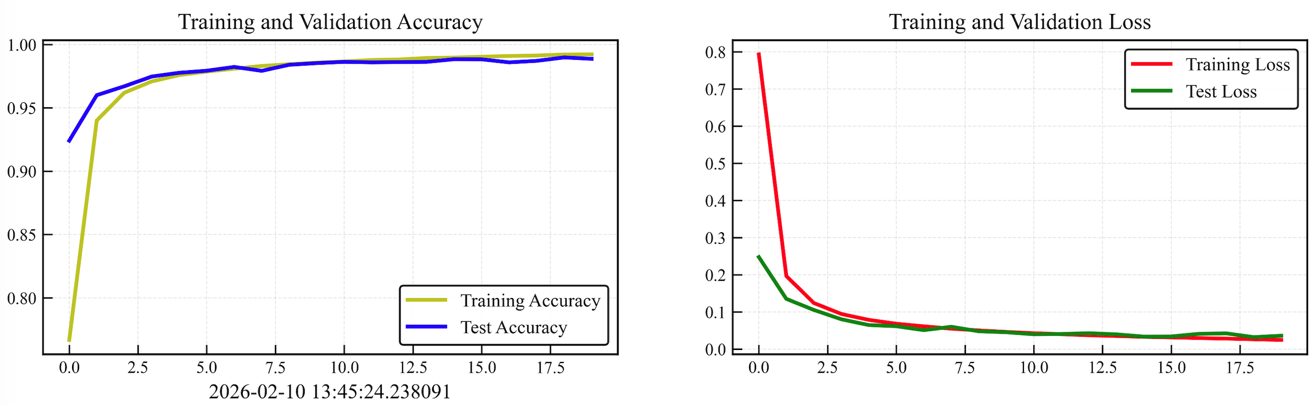

5.2 结果分析

从训练曲线可以看出：

训练准确率：从77.9%快速上升到99.3%，说明模型能够很好地学习训练数据的特征。
测试准确率：最终达到99.0%，表明模型具有良好的泛化能力，没有出现严重的过拟合。
损失函数：训练损失和测试损失都随着训练逐渐下降并趋于稳定，说明优化过程是有效的。
收敛性：模型在大约10个epoch后基本收敛，后续训练主要是微调。

六、总结与展望

通过本次实验，我们完成了以下工作：

数据准备：成功加载并预处理了MNIST手写数字数据集。
模型构建：设计并实现了一个简单的卷积神经网络。
模型训练：使用PyTorch完成了模型的训练和验证。
结果分析：模型在测试集上达到了99.0%的准确率。

关键收获：

CNN在图像分类任务中具有显著优势
合理的网络设计和参数选择对模型性能至关重要
数据预处理和增强可以提升模型泛化能力

进一步探索方向：

尝试更复杂的网络结构（如ResNet、VGG等）
使用其他数据集（如CIFAR-10、Fashion-MNIST）进行测试
实现模型部署到移动端或Web端
探索模型的可解释性方法