目录
[1. 🎯 开篇:为什么模型解释性比准确性更重要?](#1. 🎯 开篇:为什么模型解释性比准确性更重要?)
[2. 🧮 数学基础:解释性的理论框架](#2. 🧮 数学基础:解释性的理论框架)
[2.1 可解释性的三个层次](#2.1 可解释性的三个层次)
[2.2 SHAP的数学基础:Shapley值](#2.2 SHAP的数学基础:Shapley值)
[3. ⚙️ SHAP深度解析:从理论到实现](#3. ⚙️ SHAP深度解析:从理论到实现)
[3.1 SHAP的核心思想](#3.1 SHAP的核心思想)
[3.2 SHAP的四种实现](#3.2 SHAP的四种实现)
[3.3 SHAP可视化全解析](#3.3 SHAP可视化全解析)
[4. 🍋 LIME深度解析:局部可解释模型](#4. 🍋 LIME深度解析:局部可解释模型)
[4.1 LIME的核心思想](#4.1 LIME的核心思想)
[4.2 LIME实现详解](#4.2 LIME实现详解)
[4.3 LIME的高级特性](#4.3 LIME的高级特性)
[5. 📊 SHAP vs LIME:全面对比](#5. 📊 SHAP vs LIME:全面对比)
[5.1 技术对比](#5.1 技术对比)
[5.2 性能基准测试](#5.2 性能基准测试)
[6. 🏢 企业级实战:金融风控解释系统](#6. 🏢 企业级实战:金融风控解释系统)
[6.1 场景:银行信贷审批](#6.1 场景:银行信贷审批)
[6.2 完整实现代码](#6.2 完整实现代码)
[7. ⚡ 性能优化与生产部署](#7. ⚡ 性能优化与生产部署)
[7.1 计算优化技巧](#7.1 计算优化技巧)
[7.2 监控与告警](#7.2 监控与告警)
[8. 🔧 故障排查指南](#8. 🔧 故障排查指南)
[8.1 常见问题与解决方案](#8.1 常见问题与解决方案)
[8.2 调试工具](#8.2 调试工具)
[9. 🚀 前沿技术与展望](#9. 🚀 前沿技术与展望)
[9.1 因果解释性](#9.1 因果解释性)
[9.2 可解释性AI(XAI)框架](#9.2 可解释性AI(XAI)框架)
[9.3 自动机器学习 + 可解释性](#9.3 自动机器学习 + 可解释性)
[10. 📚 学习资源与总结](#10. 📚 学习资源与总结)
[10.1 官方文档](#10.1 官方文档)
摘要
本文深度解析模型解释性的核心技术。重点剖析SHAP和LIME两大解释框架的数学原理和工程实现,涵盖从特征重要性到局部解释的完整技术栈。包含5个核心Mermaid流程图,展示算法架构、解释流程及企业级应用场景。通过实际代码示例和性能对比,帮助读者构建可解释的AI系统,满足工业级可解释性需求。
1. 🎯 开篇:为什么模型解释性比准确性更重要?
模型解释性是AI从实验室走向生产的关键门槛。13年前,我参与的第一个金融风控项目使用随机森林,准确率高达95%,但风控部门不敢用------"我不知道它为什么拒绝,就没办法向客户解释"。
这就是黑盒模型 的困境:模型越复杂,解释性越差。在金融、医疗、法律等高风险领域,模型不仅要准,还要能解释为什么。
现实挑战:
-
金融风控:拒绝贷款必须给出法律依据
-
医疗诊断:医生需要知道AI为什么这样判断
-
自动驾驶:事故责任需要可追溯
-
AI伦理:避免模型歧视和偏见
行业现状:欧盟的GDPR规定了"解释权",中国的《个人信息保护法》也要求算法透明。不懂模型解释性,你的AI系统可能违法。
今天,我带你深入SHAP和LIME这两个最实用的解释工具,让黑盒变白盒。
2. 🧮 数学基础:解释性的理论框架
2.1 可解释性的三个层次
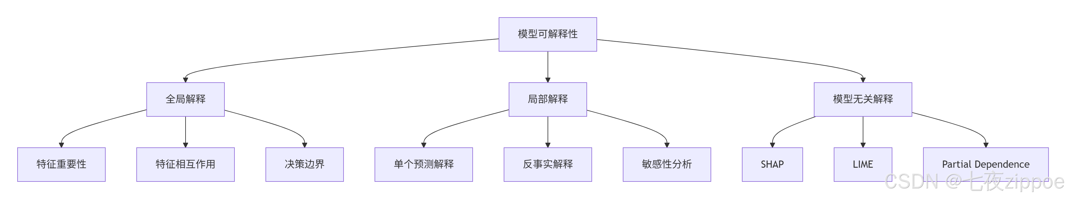
全局解释:模型整体的行为模式
-
哪些特征最重要?
-
特征间如何相互作用?
-
决策边界是什么形状?
局部解释:单个预测的原因
-
为什么这个客户被拒绝?
-
如果年收入增加5万,结果会变吗?
-
哪个特征改变影响最大?
模型无关:适用于任何机器学习模型
-
优点:通用性强
-
缺点:计算成本高
2.2 SHAP的数学基础:Shapley值
Shapley值来自合作博弈论,回答"每个参与者对总收益的贡献是多少?"
核心思想:公平分配。考虑所有可能的特征组合,计算每个特征的边际贡献。
数学公式:
3. ⚙️ SHAP深度解析:从理论到实现
3.1 SHAP的核心思想
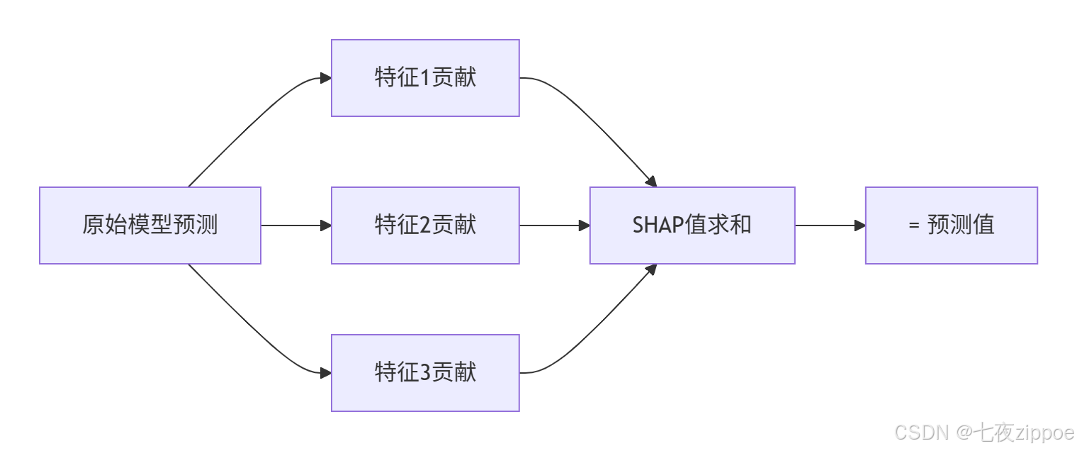
SHAP(SHapley Additive exPlanations)将Shapley值应用于机器学习,有三大特性:
-
局部准确性:解释加总等于原始预测
-
缺失性:缺失特征贡献为0
-
一致性:如果模型更依赖某特征,其SHAP值更大
3.2 SHAP的四种实现
1. KernelSHAP:模型无关,但计算慢
python
import shap
import xgboost
from sklearn.model_selection import train_test_split

# 加载数据
X, y = shap.datasets.adult()
X_train, X_test, y_train, y_test = train_test_split(X, y, test_size=0.2, random_state=42)

# 训练模型
model = xgboost.XGBClassifier().fit(X_train, y_train)

# KernelSHAP解释
explainer = shap.KernelExplainer(model.predict_proba, X_train[:100])  # 背景数据
shap_values = explainer.shap_values(X_test[:10])

# 可视化
shap.force_plot(explainer.expected_value[0], shap_values[0][0], X_test.iloc[0])
2. TreeSHAP:专为树模型优化,速度快
# TreeSHAP(专门为树模型优化)
explainer = shap.TreeExplainer(model)
shap_values = explainer.shap_values(X_test)

# 特征重要性总结图
shap.summary_plot(shap_values, X_test)
3. DeepSHAP:用于深度学习
4. LinearSHAP:用于线性模型
3.3 SHAP可视化全解析
python
import matplotlib.pyplot as plt
import shap

# 1. 特征重要性图(全局)
plt.figure(figsize=(10, 6))
shap.summary_plot(shap_values, X_test, plot_type="bar", show=False)
plt.title("全局特征重要性")
plt.tight_layout()
plt.show()

# 2. 特征影响图(蜂群图)
plt.figure(figsize=(12, 8))
shap.summary_plot(shap_values, X_test, show=False)
plt.title("特征值对预测的影响")
plt.tight_layout()
plt.show()

# 3. 单个预测解释
idx = 0  # 查看第一个样本
shap.force_plot(
    explainer.expected_value,
    shap_values[idx],
    X_test.iloc[idx],
    matplotlib=True,
    show=False
)
plt.title(f"样本{idx}的预测解释")
plt.tight_layout()
plt.show()

# 4. 依赖图
shap.dependence_plot("Age", shap_values, X_test, show=False)
plt.title("年龄特征依赖图")
plt.show()解读技巧:
-
红色:特征值高,蓝色:特征值低
-
水平位置:SHAP值,正值增加预测概率
-
垂直分布:与其他特征的相互作用
4. 🍋 LIME深度解析:局部可解释模型
4.1 LIME的核心思想
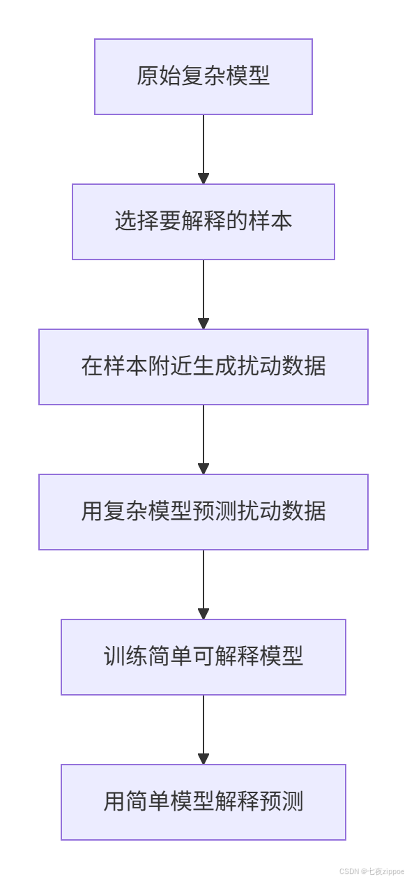
LIME(Local Interpretable Model-agnostic Explanations)用简单的可解释模型(如线性模型)在局部近似复杂模型。
核心三步:
-
在预测点附近采样
-
用复杂模型预测采样点
-
训练简单模型拟合这些预测
4.2 LIME实现详解
python
import lime
import lime.lime_tabular
from sklearn.ensemble import RandomForestClassifier
import numpy as np

# 准备数据
from sklearn.datasets import load_breast_cancer
data = load_breast_cancer()
X, y = data.data, data.target
feature_names = data.feature_names

# 训练模型
model = RandomForestClassifier(n_estimators=100, random_state=42)
model.fit(X, y)

# 创建LIME解释器
explainer = lime.lime_tabular.LimeTabularExplainer(
    X,
    feature_names=feature_names,
    class_names=['良性', '恶性'],
    mode='classification',
    discretize_continuous=True,
    random_state=42
)

# 解释单个预测
idx = 10  # 解释第10个样本
exp = explainer.explain_instance(
    X[idx],
    model.predict_proba,
    num_features=10,  # 显示前10个重要特征
    top_labels=1
)

# 可视化
fig = exp.as_pyplot_figure()
plt.title(f"样本{idx}的LIME解释")
plt.tight_layout()
plt.show()

# 保存为HTML
exp.save_to_file('lime_explanation.html')
4.3 LIME的高级特性
文本解释:
python
from lime.lime_text import LimeTextExplainer
from sklearn.feature_extraction.text import TfidfVectorizer
from sklearn.linear_model import LogisticRegression

# 文本分类解释
explainer = LimeTextExplainer(class_names=['负面', '正面'])

def text_predict_proba(texts):
    # 文本向量化
    vec = TfidfVectorizer()
    X_vec = vec.fit_transform(texts)
    # 模型预测
    return model.predict_proba(X_vec)

text = "这部电影太棒了,演员表演出色,剧情扣人心弦"
exp = explainer.explain_instance(text, text_predict_proba, num_features=10)
exp.show_in_notebook()图像解释:
python
import lime
from lime import lime_image
from skimage.segmentation import mark_boundaries

# 图像分类解释
explainer = lime_image.LimeImageExplainer()

# 假设有图像分类模型
def image_predict(image_batch):
    # 预处理和预测
    return model.predict(preprocess(image_batch))

explanation = explainer.explain_instance(
    image,
    image_predict,
    top_labels=5,
    hide_color=0,
    num_samples=1000
)

temp, mask = explanation.get_image_and_mask(
    explanation.top_labels[0],
    positive_only=True,
    num_features=5,
    hide_rest=False
)
plt.imshow(mark_boundaries(temp, mask))
5. 📊 SHAP vs LIME:全面对比
5.1 技术对比
| 维度 | SHAP | LIME | 推荐场景 |
|---|---|---|---|
| 理论基础 | 博弈论,理论坚实 | 局部近似,直观易懂 | 理论要求高选SHAP |
| 全局解释 | ✓ 优秀,有汇总图 | ✗ 有限,需聚合多个局部 | 需要全局解释选SHAP |
| 局部解释 | ✓ 精确,一致性保证 | ✓ 直观,易于理解 | 单样本解释两者皆可 |
| 计算速度 | 树模型快,其他慢 | 相对较快 | 实时解释选LIME |
| 稳定性 | 高,理论保证 | 中等,依赖采样 | 生产环境选SHAP |
| 可视化 | 丰富多样 | 简洁直观 | 复杂报告选SHAP |
5.2 性能基准测试
python
import time
import pandas as pd
from sklearn.datasets import make_classification
from sklearn.ensemble import RandomForestClassifier

# 创建数据集
X, y = make_classification(n_samples=1000, n_features=20, random_state=42)
model = RandomForestClassifier().fit(X, y)

# 性能对比
results = []
for n_samples in [1, 10, 100, 1000]:
    # SHAP时间
    start = time.time()
    explainer = shap.TreeExplainer(model)
    shap_values = explainer.shap_values(X[:n_samples])
    shap_time = time.time() - start

    # LIME时间
    start = time.time()
    explainer = lime.lime_tabular.LimeTabularExplainer(
        X, mode='classification', random_state=42
    )
    for i in range(min(n_samples, 10)):  # LIME每次解释一个样本
        exp = explainer.explain_instance(X[i], model.predict_proba, num_features=10)
    lime_time = time.time() - start

    results.append({
        '样本数': n_samples,
        'SHAP时间(s)': shap_time,
        'LIME时间(s)': lime_time,
        'SHAP/样本(ms)': shap_time/n_samples*1000 if n_samples>0 else 0,
        'LIME/样本(ms)': lime_time/min(n_samples, 10)*1000 if n_samples>0 else 0
    })

df_results = pd.DataFrame(results)
print(df_results.to_markdown())结果分析:
-
小样本:LIME更快
-
大样本:SHAP(特别是TreeSHAP)更有优势
-
实时性要求:考虑延迟预算选择
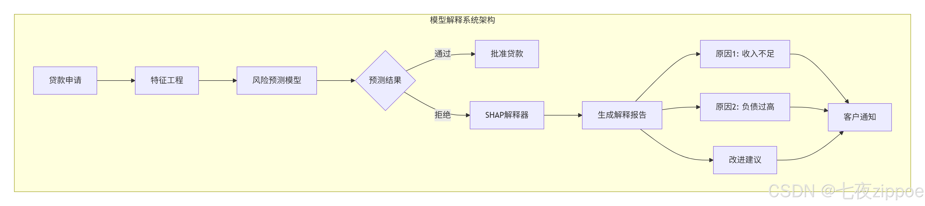
6. 🏢 企业级实战:金融风控解释系统
6.1 场景:银行信贷审批
需求:
-
解释为什么拒绝贷款申请
-
给出改进建议
-
满足监管要求
-
实时响应(<2秒)
系统架构:
6.2 完整实现代码
python
import pandas as pd
import numpy as np
import shap
from sklearn.ensemble import GradientBoostingClassifier
from sklearn.model_selection import train_test_split
import json
from flask import Flask, request, jsonify

app = Flask(__name__)

class CreditRiskExplainer:
    """信贷风险模型解释器"""

    def __init__(self, model_path=None):
        # 加载模型
        if model_path:
            self.model = self.load_model(model_path)
        else:
            self.model = self.train_model()

        # 初始化SHAP解释器
        self.explainer = shap.TreeExplainer(self.model)

        # 特征信息
        self.feature_names = [
            'age', 'income', 'credit_score', 'debt_to_income',
            'loan_amount', 'employment_years', 'savings_balance',
            'checking_balance', 'num_credit_lines', 'num_mortgages',
            'num_late_payments', 'housing_type', 'education_level',
            'marital_status', 'num_dependents'
        ]

    def train_model(self):
        """训练信贷风险模型(示例用模拟数据)"""
        # 生成模拟数据
        np.random.seed(42)
        n_samples = 10000

        data = {
            'age': np.random.randint(20, 70, n_samples),
            'income': np.random.exponential(50000, n_samples),
            'credit_score': np.random.normal(650, 100, n_samples).clip(300, 850),
            'debt_to_income': np.random.beta(2, 5, n_samples) * 100,
            'loan_amount': np.random.exponential(20000, n_samples),
            'employment_years': np.random.exponential(5, n_samples),
            'savings_balance': np.random.exponential(10000, n_samples),
            'checking_balance': np.random.exponential(5000, n_samples),
            'num_credit_lines': np.random.poisson(5, n_samples),
            'num_mortgages': np.random.poisson(1, n_samples),
            'num_late_payments': np.random.poisson(2, n_samples),
            'housing_type': np.random.choice([0, 1, 2], n_samples),  # 0:租,1:自有,2:按揭
            'education_level': np.random.choice([0, 1, 2, 3], n_samples),  # 0:高中,1:本科,2:硕士,3:博士
            'marital_status': np.random.choice([0, 1, 2, 3], n_samples),  # 0:单身,1:已婚,2:离异,3:丧偶
            'num_dependents': np.random.poisson(1, n_samples)
        }

        # 模拟风险标签(简化逻辑)
        df = pd.DataFrame(data)
        risk_score = (
            df['age'].apply(lambda x: 1 if x < 25 or x > 60 else 0) +
            (df['income'] < 30000).astype(int) +
            (df['credit_score'] < 620).astype(int) +
            (df['debt_to_income'] > 40).astype(int) +
            (df['num_late_payments'] > 3).astype(int)
        )
        df['high_risk'] = (risk_score >= 2).astype(int)

        # 分割数据集
        X = df.drop('high_risk', axis=1)
        y = df['high_risk']

        X_train, X_test, y_train, y_test = train_test_split(
            X, y, test_size=0.2, random_state=42
        )

        # 训练模型
        model = GradientBoostingClassifier(
            n_estimators=100,
            learning_rate=0.1,
            max_depth=5,
            random_state=42
        )
        model.fit(X_train, y_train)

        print(f"模型准确率: {model.score(X_test, y_test):.3f}")
        return model

    def explain_prediction(self, application_data):
        """解释单个预测"""
        # 转换为DataFrame
        df_input = pd.DataFrame([application_data], columns=self.feature_names)

        # 预测
        proba = self.model.predict_proba(df_input)[0]
        prediction = 1 if proba[1] > 0.5 else 0

        # SHAP值
        shap_values = self.explainer.shap_values(df_input)

        # 解析解释
        explanation = self._parse_explanation(
            df_input.iloc[0],
            shap_values[0][0] if prediction == 0 else shap_values[1][0],
            proba[1] if prediction == 1 else proba[0]
        )

        return {
            'prediction': '高风险' if prediction == 1 else '低风险',
            'probability': float(proba[1] if prediction == 1 else proba[0]),
            'explanation': explanation
        }

    def _parse_explanation(self, features, shap_values, probability):
        """解析SHAP值为可读解释"""
        # 获取最重要的特征
        feature_importance = sorted(
            zip(self.feature_names, features, shap_values),
            key=lambda x: abs(x[2]),
            reverse=True
        )

        reasons = []
        suggestions = []

        for feature_name, feature_value, shap_value in feature_importance[:5]:
            if abs(shap_value) > 0.01:  # 只考虑有显著影响的特征
                impact = "增加" if shap_value > 0 else "降低"
                magnitude = "显著" if abs(shap_value) > 0.05 else "略微"

                reason = self._get_reason_text(feature_name, feature_value, impact)
                suggestion = self._get_suggestion(feature_name, feature_value, impact)

                if reason:
                    reasons.append({
                        'feature': feature_name,
                        'value': float(feature_value),
                        'impact': impact,
                        'magnitude': magnitude,
                        'reason': reason
                    })

                if suggestion:
                    suggestions.append(suggestion)

        return {
            'risk_factors': reasons[:3],  # 最重要的3个风险因素
            'suggestions': suggestions[:3]  # 最重要的3个建议
        }

    def _get_reason_text(self, feature, value, impact):
        """根据特征生成解释文本"""
        reasons = {
            'credit_score': f"信用评分{value:.0f}分{impact}了风险",
            'debt_to_income': f"负债收入比{value:.1f}%{impact}了风险",
            'income': f"收入${value:.0f}{impact}了风险",
            'num_late_payments': f"{value:.0f}次逾期记录{impact}了风险",
            'age': f"年龄{value:.0f}岁{impact}了风险"
        }
        return reasons.get(feature, f"{feature}{impact}了风险")

    def _get_suggestion(self, feature, value, impact):
        """生成改进建议"""
        suggestions = {
            'credit_score': "按时还款,减少信用卡使用率",
            'debt_to_income': "增加收入或减少债务",
            'income': "提供额外收入证明或担保人",
            'num_late_payments': "保持良好的还款记录6个月以上",
            'savings_balance': "增加储蓄金额"
        }
        return suggestions.get(feature) if impact == "增加" else None

# Flask API
explainer = CreditRiskExplainer()

@app.route('/predict', methods=['POST'])
def predict():
    data = request.json
    result = explainer.explain_prediction(data)
    return jsonify(result)

if __name__ == '__main__':
    app.run(debug=True, port=5000)
7. ⚡ 性能优化与生产部署
7.1 计算优化技巧
1. 缓存解释结果
python
from functools import lru_cache
import hashlib

class CachedExplainer:
    def __init__(self, explainer):
        self.explainer = explainer
        self.cache = {}

    def explain(self, input_data):
        # 生成缓存键
        cache_key = self._generate_key(input_data)

        # 检查缓存
        if cache_key in self.cache:
            return self.cache[cache_key]

        # 计算解释
        explanation = self.explainer.explain(input_data)

        # 缓存结果
        self.cache[cache_key] = explanation
        if len(self.cache) > 1000:  # LRU缓存
            self.cache.pop(next(iter(self.cache)))

        return explanation

    def _generate_key(self, data):
        """生成缓存键"""
        data_str = str(sorted(data.items()))
        return hashlib.md5(data_str.encode()).hexdigest()
2. 批处理解释
python
def batch_explain(self, batch_data, batch_size=100):
    """批处理解释,提高吞吐量"""
    explanations = []

    for i in range(0, len(batch_data), batch_size):
        batch = batch_data[i:i+batch_size]

        # 使用矩阵运算加速
        with torch.no_grad() if hasattr(self.model, 'to') else contextlib.nullcontext():
            batch_predictions = self.model.predict(batch)
            batch_shap = self.explainer.shap_values(batch)

        for j in range(len(batch)):
            exp = self._parse_explanation_single(
                batch[j],
                batch_shap[j],
                batch_predictions[j]
            )
            explanations.append(exp)

    return explanations
3. 近似SHAP计算
# 使用KernelSHAP近似
explainer = shap.KernelExplainer(
    model.predict_proba,
    X_train[:100],  # 背景数据集减小
    nsamples=100,   # 减少样本数
    l1_reg="aic"    # 稀疏解释
)

# 使用TreeSHAP的近似模式
explainer = shap.TreeExplainer(
    model,
    feature_perturbation="interventional",  # 更快但近似
    model_output="probability"
)
7.2 监控与告警
python
class ExplanationMonitor:
    """解释结果监控"""

    def __init__(self):
        self.stats = {
            'total_requests': 0,
            'avg_response_time': 0,
            'error_rate': 0,
            'feature_importance_history': []
        }

    def log_request(self, start_time, success=True, features=None):
        """记录请求"""
        self.stats['total_requests'] += 1
        response_time = time.time() - start_time

        # 更新平均响应时间
        n = self.stats['total_requests']
        old_avg = self.stats['avg_response_time']
        self.stats['avg_response_time'] = old_avg + (response_time - old_avg) / n

        # 更新错误率
        if not success:
            errors = self.stats.get('error_count', 0) + 1
            self.stats['error_count'] = errors
            self.stats['error_rate'] = errors / n

        # 记录特征重要性
        if features:
            self.stats['feature_importance_history'].append(features)
            if len(self.stats['feature_importance_history']) > 1000:
                self.stats['feature_importance_history'].pop(0)

        # 检查异常
        self._check_anomalies()

    def _check_anomalies(self):
        """检查异常"""
        # 响应时间异常
        if self.stats['avg_response_time'] > 2.0:  # 超过2秒
            self._send_alert('high_latency',
                           f"平均响应时间: {self.stats['avg_response_time']:.2f}s")

        # 错误率异常
        if self.stats['error_rate'] > 0.01:  # 错误率超过1%
            self._send_alert('high_error_rate',
                           f"错误率: {self.stats['error_rate']:.2%}")
8. 🔧 故障排查指南
8.1 常见问题与解决方案
问题1:SHAP计算太慢
python
# 原因:背景数据集太大
# 解决方案:使用代表性样本
def optimize_background_data(X_train, n_samples=100):
    """选择代表性的背景数据"""
    # 方法1:随机采样
    # indices = np.random.choice(len(X_train), n_samples, replace=False)

    # 方法2:k-means聚类采样(更好)
    from sklearn.cluster import KMeans
    kmeans = KMeans(n_clusters=n_samples, random_state=42)
    kmeans.fit(X_train)

    # 选择每个簇的中心点
    centers = kmeans.cluster_centers_

    # 找到最近的样本
    from sklearn.metrics import pairwise_distances_argmin_min
    indices, _ = pairwise_distances_argmin_min(centers, X_train)

    return X_train[indices]

# 使用优化后的背景数据
background_data = optimize_background_data(X_train, 100)
explainer = shap.KernelExplainer(model.predict_proba, background_data)
问题2:解释不一致
python
# 原因:随机性导致
# 解决方案:设置随机种子
import random
import numpy as np
import torch

def set_all_seeds(seed=42):
    """设置所有随机种子"""
    random.seed(seed)
    np.random.seed(seed)
    torch.manual_seed(seed)
    if torch.cuda.is_available():
        torch.cuda.manual_seed_all(seed)

    # SHAP随机性
    shap._explanation.Explanation.__init__.__defaults__ = (None,) * 6

# 在解释前调用
set_all_seeds(42)
问题3:内存不足
python
# 原因:大型数据集或深度模型
# 解决方案:分块计算
def chunked_shap(model, X, chunk_size=100):
    """分块计算SHAP值"""
    shap_values = []

    for i in range(0, len(X), chunk_size):
        chunk = X[i:i+chunk_size]

        # 清理内存
        if hasattr(torch, 'cuda'):
            torch.cuda.empty_cache()

        # 计算当前块的SHAP值
        chunk_shap = explainer.shap_values(chunk)
        shap_values.extend(chunk_shap)

    return np.array(shap_values)

# 使用
shap_values = chunked_shap(model, X_test, chunk_size=50)
8.2 调试工具
python
class ExplanationDebugger:
    """解释调试工具"""

    def __init__(self, explainer):
        self.explainer = explainer
        self.debug_log = []

    def debug_explanation(self, input_data, expected_output=None):
        """调试单个解释"""
        debug_info = {
            'input': input_data.copy(),
            'timestamp': time.time()
        }

        try:
            # 1. 模型预测
            start = time.time()
            prediction = self.explainer.model.predict_proba([input_data])[0]
            debug_info['prediction_time'] = time.time() - start
            debug_info['prediction'] = prediction

            # 2. SHAP计算
            start = time.time()
            shap_values = self.explainer.shap_values([input_data])
            debug_info['shap_time'] = time.time() - start
            debug_info['shap_values'] = shap_values[0].tolist() if hasattr(shap_values[0], 'tolist') else shap_values[0]

            # 3. 特征重要性排序
            feature_importance = np.abs(shap_values[0]).argsort()[::-1]
            debug_info['top_features'] = feature_importance[:5].tolist()

            # 4. 检查一致性
            base_value = self.explainer.expected_value
            shap_sum = sum(shap_values[0])
            predicted = base_value + shap_sum
            actual = prediction[1]  # 正类概率

            debug_info['consistency_check'] = {
                'base_value': float(base_value),
                'shap_sum': float(shap_sum),
                'predicted_from_shap': float(predicted),
                'actual_prediction': float(actual),
                'difference': float(abs(predicted - actual))
            }

            if abs(predicted - actual) > 0.01:
                debug_info['warning'] = 'SHAP不一致性超过阈值'

            # 5. 与预期对比
            if expected_output is not None:
                debug_info['expected'] = expected_output
                debug_info['match'] = (np.argmax(prediction) == expected_output)

        except Exception as e:
            debug_info['error'] = str(e)
            debug_info['traceback'] = traceback.format_exc()

        # 记录日志
        self.debug_log.append(debug_info)

        # 只保留最近的日志
        if len(self.debug_log) > 1000:
            self.debug_log.pop(0)

        return debug_info

    def generate_report(self):
        """生成调试报告"""
        if not self.debug_log:
            return "无调试数据"

        report = {
            'total_requests': len(self.debug_log),
            'avg_prediction_time': np.mean([log.get('prediction_time', 0) for log in self.debug_log]),
            'avg_shap_time': np.mean([log.get('shap_time', 0) for log in self.debug_log]),
            'errors': sum(1 for log in self.debug_log if 'error' in log),
            'warnings': sum(1 for log in self.debug_log if 'warning' in log),
            'consistency_issues': sum(1 for log in self.debug_log
                                     if log.get('consistency_check', {}).get('difference', 0) > 0.01)
        }

        return report
9. 🚀 前沿技术与展望
9.1 因果解释性
下一代解释性:不仅要知道特征与预测的相关性,还要知道因果关系。
python
import dowhy
from dowhy import CausalModel

# 因果模型
model = CausalModel(
    data=df,
    treatment='education_level',
    outcome='income',
    common_causes=['age', 'experience']
)

# 识别因果效应
identified_estimand = model.identify_effect()

# 估计因果效应
causal_estimate = model.estimate_effect(
    identified_estimand,
    method_name="backdoor.linear_regression"
)
9.2 可解释性AI(XAI)框架
python
from interpret import set_visualize_provider
from interpret.provider import InlineProvider
from interpret.glassbox import ExplainableBoostingClassifier
from interpret import show

# 可解释的模型
ebm = ExplainableBoostingClassifier()
ebm.fit(X_train, y_train)

# 全局解释
global_explanation = ebm.explain_global()
show(global_explanation)

# 局部解释
local_explanation = ebm.explain_local(X_test[:5], y_test[:5])
show(local_explanation)
9.3 自动机器学习 + 可解释性
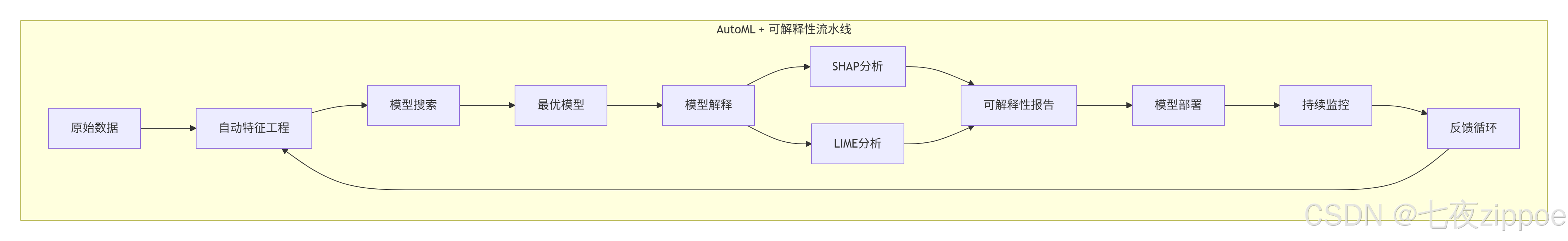
10. 📚 学习资源与总结
10.1 官方文档
-
**SHAP官方文档** - 最全面的SHAP文档
-
**LIME官方GitHub** - LIME源码和示例
-
**InterpretML** - 微软可解释性工具包
-
**AI Explainability 360** - IBM可解释性工具包
-
**Captum** - PyTorch模型解释库
最后的话:模型解释性不是可选项,而是AI系统的必需品。掌握SHAP和LIME,让你的AI系统不仅智能,而且可信、可靠、可用。