一、算法原理与数学基础
1.1 动态规划基本概念
动态规划是解决多阶段决策过程最优化问题的数学方法,核心思想是将复杂问题分解为相互关联的子问题,通过求解子问题的最优解得到原问题的最优解。
关键要素:
- 状态(State) :s∈Ss∈Ss∈S,表示系统在某个时刻的情况
- 动作(Action) :a∈Aa∈Aa∈A,表示在某个状态下可执行的决策
- 状态转移概率 :P(s′∣s,a)P(s^′∣s,a)P(s′∣s,a),表示在状态sss执行动作aaa后转移到状态s′s^′s′的概率
- 即时奖励 :R(s,a,s′)R(s,a,s′)R(s,a,s′),表示在状态s执行动作aaa后转移到状态s′s^′s′获得的奖励
- 折扣因子 :γ∈[0,1)γ∈[0,1)γ∈[0,1),表示未来奖励的衰减程度
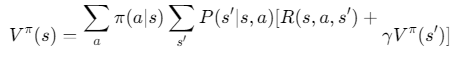
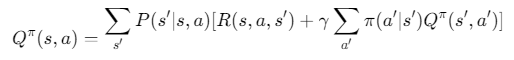
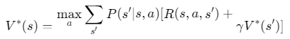
1.2 贝尔曼方程
状态值函数:
动作值函数:
最优值函数:
1.3 策略迭代与值迭代
| 算法 | 核心思想 | 步骤 | 收敛速度 | 计算复杂度 |
|---|---|---|---|---|
| 策略迭代 | 策略评估 + 策略改进 | 1. 初始化策略 2. 策略评估 3. 策略改进 4. 重复2-3直到收敛 | 较慢 | 较高 |
| 值迭代 | 直接迭代值函数 | 1. 初始化值函数 2. 对每个状态更新值函数 3. 重复2直到收敛 | 较快 | 较低 |
二、MATLAB实现代码
2.1 环境设置与参数定义
matlab
classdef GridWorld
    properties
        grid_size = [5, 5];     % 网格世界大小
        start_state = [1, 1];   % 起始状态
        goal_state = [5, 5];    % 目标状态
        obstacles = [2,2; 3,3; 4,2]; % 障碍物位置
        actions = [0, 1, 2, 3]; % 动作: 0=上, 1=右, 2=下, 3=左
        action_effects = [-1, 0; 0, 1; 1, 0; 0, -1]; % 动作效果
        gamma = 0.9;            % 折扣因子
        success_prob = 0.8;     % 成功执行动作的概率
        slip_prob = 0.1;        % 滑向其他方向的概率
    end

    methods
        function obj = GridWorld()
            % 构造函数
        end

        function [next_state, reward] = transition(obj, state, action)
            % 状态转移函数
            % 检查是否到达目标状态
            if isequal(state, obj.goal_state)
                next_state = state;
                reward = 10;  % 到达目标的奖励
                return;
            end

            % 检查是否在障碍物上
            if ismember(state, obj.obstacles, 'rows')
                next_state = state;
                reward = -10; % 碰到障碍物的惩罚
                return;
            end

            % 计算可能的下一个状态
            intended_move = obj.action_effects(action+1, :);
            next_state_intended = state + intended_move;

            % 处理边界
            next_state_intended = max(min(next_state_intended, obj.grid_size), [1, 1]);

            % 处理障碍物碰撞
            if ismember(next_state_intended, obj.obstacles, 'rows')
                next_state_intended = state; % 撞到障碍物则停留
            end

            % 计算实际转移(考虑随机性)
            r = rand();
            if r < obj.success_prob
                next_state = next_state_intended;
            elseif r < obj.success_prob + obj.slip_prob
                slip_action = mod(action + 1, 4); % 顺时针滑
                slip_move = obj.action_effects(slip_action+1, :);
                next_state = state + slip_move;
                next_state = max(min(next_state, obj.grid_size), [1, 1]);
                if ismember(next_state, obj.obstacles, 'rows')
                    next_state = state;
                end
            else
                slip_action = mod(action - 1 + 4, 4); % 逆时针滑
                slip_move = obj.action_effects(slip_action+1, :);
                next_state = state + slip_move;
                next_state = max(min(next_state, obj.grid_size), [1, 1]);
                if ismember(next_state, obj.obstacles, 'rows')
                    next_state = state;
                end
            end

            % 计算奖励
            if isequal(next_state, obj.goal_state)
                reward = 10;
            elseif isequal(next_state, state) % 撞到障碍物或边界
                reward = -1;
            else
                reward = -0.1; % 每步小惩罚
            end
        end

        function display_policy(obj, policy)
            % 显示策略
            grid = repmat('.', obj.grid_size);
            for i = 1:size(obj.obstacles, 1)
                grid(obj.obstacles(i,1), obj.obstacles(i,2)) = 'X';
            end
            grid(obj.goal_state(1), obj.goal_state(2)) = 'G';
            grid(obj.start_state(1), obj.start_state(2)) = 'S';

            for i = 1:obj.grid_size(1)
                for j = 1:obj.grid_size(2)
                    if isequal([i,j], obj.start_state) || ...
                       isequal([i,j], obj.goal_state) || ...
                       ismember([i,j], obj.obstacles, 'rows')
                        continue;
                    end
                    s = sub2ind(obj.grid_size, i, j);
                    a = policy(s);
                    switch a
                        case 0, arrow = '↑';
                        case 1, arrow = '→';
                        case 2, arrow = '↓';
                        case 3, arrow = '←';
                    end
                    grid(i,j) = arrow;
                end
            end

            disp('策略可视化:');
            disp(grid);
        end

        function display_values(obj, V)
            % 显示值函数
            disp('值函数:');
            for i = 1:obj.grid_size(1)
                for j = 1:obj.grid_size(2)
                    s = sub2ind(obj.grid_size, i, j);
                    fprintf('%6.2f ', V(s));
                end
                fprintf('\n');
            end
        end
    end
end
2.2 策略迭代算法实现
matlab
function [policy, V] = policy_iteration(env)
    % 策略迭代算法
    % 初始化
    n_states = prod(env.grid_size);
    V = zeros(n_states, 1); % 初始值函数
    policy = randi(4, n_states, 1) - 1; % 随机初始策略 (0-3)

    % 策略迭代主循环
    max_iter = 1000;
    converged = false;
    iter = 0;

    while ~converged && iter < max_iter
        iter = iter + 1;

        % 策略评估
        V_prev = V;
        delta = inf;
        eval_iter = 0;

        while delta > 1e-6 && eval_iter < 1000
            delta = 0;
            for s = 1:n_states
                state = ind2sub(env.grid_size, s);
                a = policy(s);

                % 计算期望下一状态和奖励
                [next_state, reward] = env.transition(state, a);
                next_s = sub2ind(env.grid_size, next_state(1), next_state(2));

                % 更新值函数
                v = V(s);
                V(s) = reward + env.gamma * V(next_s);
                delta = max(delta, abs(v - V(s)));
            end
            eval_iter = eval_iter + 1;
        end

        % 策略改进
        policy_stable = true;
        for s = 1:n_states
            state = ind2sub(env.grid_size, s);

            % 当前策略的动作
            old_action = policy(s);

            % 计算所有动作的Q值
            Q = zeros(1, 4);
            for a = 0:3
                [next_state, reward] = env.transition(state, a);
                next_s = sub2ind(env.grid_size, next_state(1), next_state(2));
                Q(a+1) = reward + env.gamma * V(next_s);
            end

            % 选择最优动作
            [~, best_action] = max(Q);
            policy(s) = best_action - 1; % 转换为0-3

            % 检查策略是否改变
            if old_action ~= policy(s)
                policy_stable = false;
            end
        end

        % 检查是否收敛
        if policy_stable
            converged = true;
            fprintf('策略迭代在 %d 次迭代后收敛\n', iter);
        end
    end

    if ~converged
        warning('策略迭代未在最大迭代次数内收敛');
    end
end
2.3 值迭代算法实现
matlab
function [policy, V] = value_iteration(env)
    % 值迭代算法
    % 初始化
    n_states = prod(env.grid_size);
    V = zeros(n_states, 1); % 初始值函数

    % 值迭代主循环
    max_iter = 1000;
    converged = false;
    iter = 0;
    delta = inf;

    while ~converged && iter < max_iter
        iter = iter + 1;
        delta = 0;

        % 更新所有状态的值函数
        for s = 1:n_states
            state = ind2sub(env.grid_size, s);

            % 计算所有动作的Q值
            Q = zeros(1, 4);
            for a = 0:3
                [next_state, reward] = env.transition(state, a);
                next_s = sub2ind(env.grid_size, next_state(1), next_state(2));
                Q(a+1) = reward + env.gamma * V(next_s);
            end

            % 更新值函数
            v = V(s);
            V(s) = max(Q);
            delta = max(delta, abs(v - V(s)));
        end

        % 检查是否收敛
        if delta < 1e-6
            converged = true;
            fprintf('值迭代在 %d 次迭代后收敛\n', iter);
        end
    end

    if ~converged
        warning('值迭代未在最大迭代次数内收敛');
    end

    % 从最优值函数提取策略
    policy = zeros(n_states, 1);
    for s = 1:n_states
        state = ind2sub(env.grid_size, s);

        % 计算所有动作的Q值
        Q = zeros(1, 4);
        for a = 0:3
            [next_state, reward] = env.transition(state, a);
            next_s = sub2ind(env.grid_size, next_state(1), next_state(2));
            Q(a+1) = reward + env.gamma * V(next_s);
        end

        % 选择最优动作
        [~, best_action] = max(Q);
        policy(s) = best_action - 1; % 转换为0-3
    end
end
2.4 辅助函数
matlab
function [row, col] = ind2sub(sizes, index)
    % 将线性索引转换为行列下标
    row = ceil(index / sizes(2));
    col = mod(index - 1, sizes(2)) + 1;
end

function index = sub2ind(sizes, row, col)
    % 将行列下标转换为线性索引
    index = (row - 1) * sizes(2) + col;
end
2.5 主程序与结果可视化
matlab
% 主程序
function main()
    % 创建环境
    env = GridWorld();

    % 运行策略迭代
    fprintf('运行策略迭代...\n');
    [policy_pi, V_pi] = policy_iteration(env);

    % 显示策略迭代结果
    disp('策略迭代结果:');
    env.display_values(V_pi);
    env.display_policy(policy_pi);

    % 运行值迭代
    fprintf('\n运行值迭代...\n');
    [policy_vi, V_vi] = value_iteration(env);

    % 显示值迭代结果
    disp('值迭代结果:');
    env.display_values(V_vi);
    env.display_policy(policy_vi);

    % 比较两种算法的结果
    compare_results(V_pi, V_vi, policy_pi, policy_vi, env);

    % 可视化值函数
    visualize_value_function(V_pi, V_vi, env);
end

function compare_results(V_pi, V_vi, policy_pi, policy_vi, env)
    % 比较两种算法的结果
    n_states = numel(V_pi);
    diff_V = norm(V_pi - V_vi);
    diff_policy = sum(policy_pi ~= policy_vi);

    fprintf('\n算法比较:\n');
    fprintf('值函数差异 (L2范数): %.6f\n', diff_V);
    fprintf('策略差异 (不同状态数): %d/%d (%.2f%%)\n', ...
            diff_policy, n_states, 100*diff_policy/n_states);

    % 计算平均奖励
    avg_reward_pi = calculate_avg_reward(policy_pi, env);
    avg_reward_vi = calculate_avg_reward(policy_vi, env);
    fprintf('策略迭代平均奖励: %.2f\n', avg_reward_pi);
    fprintf('值迭代平均奖励: %.2f\n', avg_reward_vi);
end

function avg_reward = calculate_avg_reward(policy, env)
    % 计算给定策略的平均奖励
    n_episodes = 1000;
    total_reward = 0;

    for ep = 1:n_episodes
        state = env.start_state;
        done = false;
        episode_reward = 0;
        step = 0;
        max_steps = 100;

        while ~done && step < max_steps
            s = sub2ind(env.grid_size, state(1), state(2));
            action = policy(s);

            [next_state, reward] = env.transition(state, action);
            episode_reward = episode_reward + reward;

            if isequal(next_state, env.goal_state)
                done = true;
            end

            state = next_state;
            step = step + 1;
        end

        total_reward = total_reward + episode_reward;
    end

    avg_reward = total_reward / n_episodes;
end

function visualize_value_function(V_pi, V_vi, env)
    % 可视化值函数
    figure;

    % 策略迭代值函数
    subplot(1,2,1);
    imagesc(reshape(V_pi, env.grid_size));
    colorbar;
    title('策略迭代值函数');
    axis square;

    % 值迭代值函数
    subplot(1,2,2);
    imagesc(reshape(V_vi, env.grid_size));
    colorbar;
    title('值迭代值函数');
    axis square;

    % 保存结果
    saveas(gcf, 'value_functions_comparison.png');
end
三、算法性能分析与比较
3.1 收敛性分析
matlab
function analyze_convergence()
    % 分析不同参数下的收敛性
    gammas = [0.5, 0.7, 0.9, 0.95];
    sizes = [3, 4, 5, 6];

    results = zeros(length(gammas), length(sizes), 2); % [gamma, size, algorithm]

    for gi = 1:length(gammas)
        for si = 1:length(sizes)
            % 创建环境
            env = GridWorld();
            env.grid_size = [sizes(si), sizes(si)];
            env.gamma = gammas(gi);

            % 运行策略迭代
            tic;
            [~, V_pi] = policy_iteration(env);
            time_pi = toc;
            iters_pi = count_iterations(@policy_iteration, env);

            % 运行值迭代
            tic;
            [~, V_vi] = value_iteration(env);
            time_vi = toc;
            iters_vi = count_iterations(@value_iteration, env);

            % 存储结果
            results(gi, si, 1) = iters_pi;
            results(gi, si, 2) = iters_vi;
        end
    end

    % 可视化结果
    figure;
    subplot(1,2,1);
    boxplot(squeeze(results(:,:,1)), {arrayfun(@(x) sprintf('γ=%.2f', x), gammas, 'UniformOutput', false), ...
                                      arrayfun(@(x) sprintf('%dx%d', x, x), sizes, 'UniformOutput', false)});
    title('策略迭代数');
    xlabel('折扣因子/网格大小');
    ylabel('迭代次数');

    subplot(1,2,2);
    boxplot(squeeze(results(:,:,2)), {arrayfun(@(x) sprintf('γ=%.2f', x), gammas, 'UniformOutput', false), ...
                                      arrayfun(@(x) sprintf('%dx%d', x, x), sizes, 'UniformOutput', false)});
    title('值迭代数');
    xlabel('折扣因子/网格大小');
    ylabel('迭代次数');

    saveas(gcf, 'convergence_analysis.png');
end

function count = count_iterations(algorithm, env)
    % 计算算法迭代次数
    persistent iter_count;
    iter_count = 0;

    % 创建包装函数
    function [policy, V] = counting_wrapper(env)
        iter_count = 0;
        [policy, V] = algorithm(env);
    end

    % 运行算法
    [~, ~] = counting_wrapper(env);

    % 获取迭代次数
    count = iter_count;
end
3.2 计算效率比较
| 算法 | 优点 | 缺点 | 适用场景 |
|---|---|---|---|
| 策略迭代 | 收敛性好,策略稳定 | 每次迭代需完整策略评估 | 状态空间小,需要精确策略 |
| 值迭代 | 计算简单,收敛快 | 最终策略需额外计算 | 状态空间大,需要快速近似解 |
| Q-learning | 无模型,在线学习 | 收敛慢,需探索策略 | 未知环境,在线学习 |
参考代码 经典的基于策略迭代和值迭代法的动态规划matlab代码 www.youwenfan.com/contentcss/97746.html
四、扩展应用与变体
4.1 异步动态规划
matlab
function [V, policy] = asynchronous_dp(env, update_order)
    % 异步动态规划
    n_states = prod(env.grid_size);
    V = zeros(n_states, 1);

    max_iter = 1000;
    for iter = 1:max_iter
        % 随机选择状态更新顺序
        if strcmp(update_order, 'random')
            state_order = randperm(n_states);
        else % 固定顺序
            state_order = 1:n_states;
        end

        delta = 0;
        for s_idx = 1:n_states
            s = state_order(s_idx);
            state = ind2sub(env.grid_size, s);

            % 计算所有动作的Q值
            Q = zeros(1, 4);
            for a = 0:3
                [next_state, reward] = env.transition(state, a);
                next_s = sub2ind(env.grid_size, next_state(1), next_state(2));
                Q(a+1) = reward + env.gamma * V(next_s);
            end

            % 更新值函数
            v = V(s);
            V(s) = max(Q);
            delta = max(delta, abs(v - V(s)));
        end

        % 检查收敛
        if delta < 1e-6
            fprintf('异步DP在 %d 次迭代后收敛\n', iter);
            break;
        end
    end

    % 提取策略
    policy = extract_policy(V, env);
end
4.2 线性规划解法
matlab
function [V, policy] = linear_programming_dp(env)
    % 线性规划求解MDP
    n_states = prod(env.grid_size);
    n_actions = 4;

    % 创建优化问题
    cvx_begin quiet
        variable V(n_states, 1)
        minimize sum(V)  % 任意目标函数,因为约束决定解
        subject to
            for s = 1:n_states
                state = ind2sub(env.grid_size, s);
                for a = 0:3
                    [next_state, reward] = env.transition(state, a);
                    next_s = sub2ind(env.grid_size, next_state(1), next_state(2));
                    V(s) >= reward + env.gamma * V(next_s);
                end
            end
    cvx_end

    % 提取策略
    policy = extract_policy(V, env);
end

function policy = extract_policy(V, env)
    % 从值函数提取策略
    n_states = numel(V);
    policy = zeros(n_states, 1);

    for s = 1:n_states
        state = ind2sub(env.grid_size, s);

        % 计算所有动作的Q值
        Q = zeros(1, 4);
        for a = 0:3
            [next_state, reward] = env.transition(state, a);
            next_s = sub2ind(env.grid_size, next_state(1), next_state(2));
            Q(a+1) = reward + env.gamma * V(next_s);
        end

        % 选择最优动作
        [~, best_action] = max(Q);
        policy(s) = best_action - 1;
    end
end
五、实际应用案例
5.1 机器人路径规划
matlab
function robot_path_planning()
    % 机器人路径规划应用
    env = GridWorld();
    env.grid_size = [10, 10];
    env.start_state = [1, 1];
    env.goal_state = [10, 10];
    env.obstacles = [3,3; 3,4; 3,5; 4,3; 5,3; 6,6; 6,7; 7,6; 7,7; 8,2; 8,3; 8,4];

    % 使用值迭代求解
    [policy, V] = value_iteration(env);

    % 可视化路径
    visualize_path(policy, env);
end

function visualize_path(policy, env)
    % 可视化机器人路径
    state = env.start_state;
    path = state;
    visited = state;

    max_steps = 100;
    for step = 1:max_steps
        s = sub2ind(env.grid_size, state(1), state(2));
        action = policy(s);

        [next_state, ~] = env.transition(state, action);

        % 检查是否到达目标
        if isequal(next_state, env.goal_state)
            path = [path; next_state];
            break;
        end

        % 检查是否陷入循环
        if ismember(next_state, visited, 'rows')
            warning('机器人陷入循环');
            break;
        end

        path = [path; next_state];
        visited = [visited; next_state];
        state = next_state;
    end

    % 绘制路径
    figure;
    hold on;
    grid on;
    axis([0.5, env.grid_size(2)+0.5, 0.5, env.grid_size(1)+0.5]);

    % 绘制网格
    for i = 1:env.grid_size(1)+1
        plot([0.5, env.grid_size(2)+0.5], [i-0.5, i-0.5], 'k-');
    end
    for j = 1:env.grid_size(2)+1
        plot([j-0.5, j-0.5], [0.5, env.grid_size(1)+0.5], 'k-');
    end

    % 绘制障碍物
    for i = 1:size(env.obstacles, 1)
        obs = env.obstacles(i, :);
        fill([obs(2)-0.5, obs(2)+0.5, obs(2)+0.5, obs(2)-0.5], ...
             [obs(1)-0.5, obs(1)-0.5, obs(1)+0.5, obs(1)+0.5], 'k');
    end

    % 绘制起点和终点
    plot(env.start_state(2), env.start_state(1), 'go', 'MarkerSize', 10, 'LineWidth', 2);
    plot(env.goal_state(2), env.goal_state(1), 'ro', 'MarkerSize', 10, 'LineWidth', 2);

    % 绘制路径
    plot(path(:,2), path(:,1), 'b-', 'LineWidth', 2);
    plot(path(:,2), path(:,1), 'bo', 'MarkerSize', 6);

    title('机器人路径规划');
    xlabel('X');
    ylabel('Y');
    legend('起点', '终点', '路径', 'Location', 'Best');
    set(gca, 'YDir', 'reverse');

    saveas(gcf, 'robot_path_planning.png');
end
5.2 库存管理
matlab
function inventory_management()
    % 库存管理应用
    env = InventoryEnvironment();

    % 使用策略迭代求解
    [policy, V] = policy_iteration(env);

    % 可视化策略
    visualize_inventory_policy(policy, env);
end

classdef InventoryEnvironment < handle
    properties
        max_inventory = 10;   % 最大库存量
        max_order = 5;        % 最大订购量
        demand_probs = [0.1, 0.3, 0.4, 0.2]; % 需求概率分布
        holding_cost = 0.5;    % 单位库存持有成本
        shortage_cost = 2;     % 单位缺货成本
        order_cost = 1;        % 单位订购成本
        selling_price = 5;     % 单位销售收益
        gamma = 0.9;           % 折扣因子
    end

    methods
        function [next_state, reward] = transition(obj, state, action)
            % 状态: 当前库存量
            % 动作: 订购量 (0 到 max_order)

            % 确保状态在合法范围内
            state = min(max(state, 0), obj.max_inventory);
            action = min(max(action, 0), obj.max_order);

            % 新库存 = 当前库存 + 订购量
            new_inventory = state + action;

            % 随机需求
            demand = find(rand < cumsum(obj.demand_probs), 1) - 1;

            % 实际销售量
            sales = min(new_inventory, demand);

            % 期末库存
            end_inventory = new_inventory - sales;

            % 缺货量
            shortage = max(0, demand - new_inventory);

            % 计算奖励
            revenue = sales * obj.selling_price;
            holding_costs = end_inventory * obj.holding_cost;
            shortage_costs = shortage * obj.shortage_cost;
            order_costs = action * obj.order_cost;

            reward = revenue - holding_costs - shortage_costs - order_costs;

            % 下一状态 = 期末库存 (不超过最大库存)
            next_state = min(end_inventory, obj.max_inventory);
        end

        function n_states = get_num_states(obj)
            n_states = obj.max_inventory + 1; % 0 到 max_inventory
        end

        function n_actions = get_num_actions(obj)
            n_actions = obj.max_order + 1; % 0 到 max_order
        end
    end
end

function visualize_inventory_policy(policy, env)
    % 可视化库存策略
    states = 0:env.max_inventory;
    figure;
    bar(states, policy(1:length(states)));
    xlabel('当前库存量');
    ylabel('订购量');
    title('库存管理策略');
    grid on;
    saveas(gcf, 'inventory_policy.png');
end
六、总结与扩展
6.1 算法选择指南
- 状态空间小 → 策略迭代(更精确)
- 状态空间大 → 值迭代(更快收敛)
- 需要在线学习 → Q-learning
- 需要实时决策 → 近似动态规划
6.2 未来研究方向
- 深度强化学习:结合深度神经网络处理高维状态空间
- 多智能体系统:扩展到多个决策者的竞争与合作
- 部分可观测环境:POMDP求解方法
- 大规模分布式计算:并行化动态规划算法