吴恩达机器学习作业（week1-4）

公式根据吴恩达老师的课总结的

题目复制来自_cv吴彦祖

数据集（ladykaka007)：链接:https://pan.baidu.com/s/1L-Tbo3flzKplAof3fFdD1w 密码:oin0

代码跟着b站ladykaka007敲的

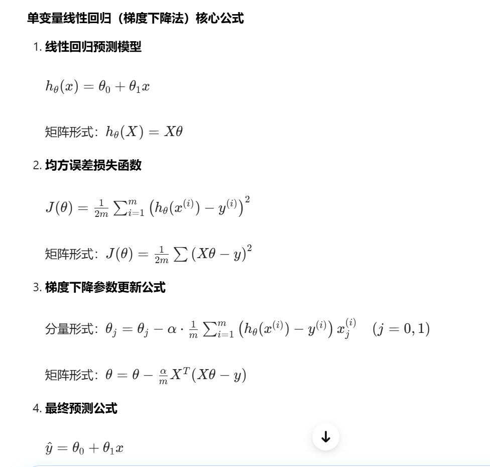
01线性回归

题目

您将使用一元线性回归来预测食品车的利润。假设你是一家特许餐厅的首席执行官，正在考虑在不同的城市开设一家新的分店。该连锁店已经在不同的城市有卡车，你有这些城市的利润和人口数据。您希望使用这些数据来帮助您选择下一个要扩展到的城市。

数据集

代码-梯度下降

import numpy as np
import pandas as pd
import matplotlib.pyplot as plt

data=pd.read_excel('D:\\小孩\\ML\\吴恩达作业\\week1线性回归\\单变量.xlsx',names=['population','profit'])
data.plot.scatter(x='population',y='profit',label='population')
plt.show()
#
data.insert(0,'ones',1)
#切片
X=data.iloc[:,0:-1]
y=data.iloc[:,-1]
X=X.values
y=y.values
y=y.reshape(90,1)

#损失函数
def costFunction(X,y,theta):
    inner=np.power(X@theta-y,2)
    return np.sum(inner)/(2*len(X))
theta=np.zeros((2,1))
cost_init=costFunction(X,y,theta)
print(cost_init)

#梯度函数
def gradientDescent(X,y,theta,alpha,iters):
    costs=[]
    for i in range(iters):
        theta=theta-(X.T@(X@theta-y))*alpha/len(X)
        cost=costFunction(X,y,theta)
        costs.append(cost)
        if i%100==0:
            print(cost)
    return theta,costs

alpha=0.02
iters=2000
theta,costs=gradientDescent(X,y,theta,alpha,iters)

#损失函数图像
fig,ax=plt.subplots()
ax.plot(np.arange(iters),costs)
ax.set(xlabel='iters',ylabel='cost',title='cost vs iters')
plt.show()

x=np.linspace(y.min(),y.max(),100)
y_=theta[0,0]+theta[1,0]*x
fig,ax=plt.subplots()
ax.scatter(X[:,-1],y,label='training data')
ax.plot(x,y_,'r',label='predict')
ax.legend()
ax.set(xlabel='population',ylabel='profit')
plt.show()

代码-正规化

import numpy as np
import pandas as pd
import matplotlib.pyplot as plt

data=pd.read_excel('D:\\小孩\\ML\\吴恩达作业\\week1线性回归\\单变量.xlsx',names=['population','profit'])
data.plot.scatter(x='population',y='profit',label='population')
plt.show()
#
data.insert(0,'ones',1)
#切片
X=data.iloc[:,0:-1]
y=data.iloc[:,-1]
X=X.values
y=y.values
y=y.reshape(90,1)

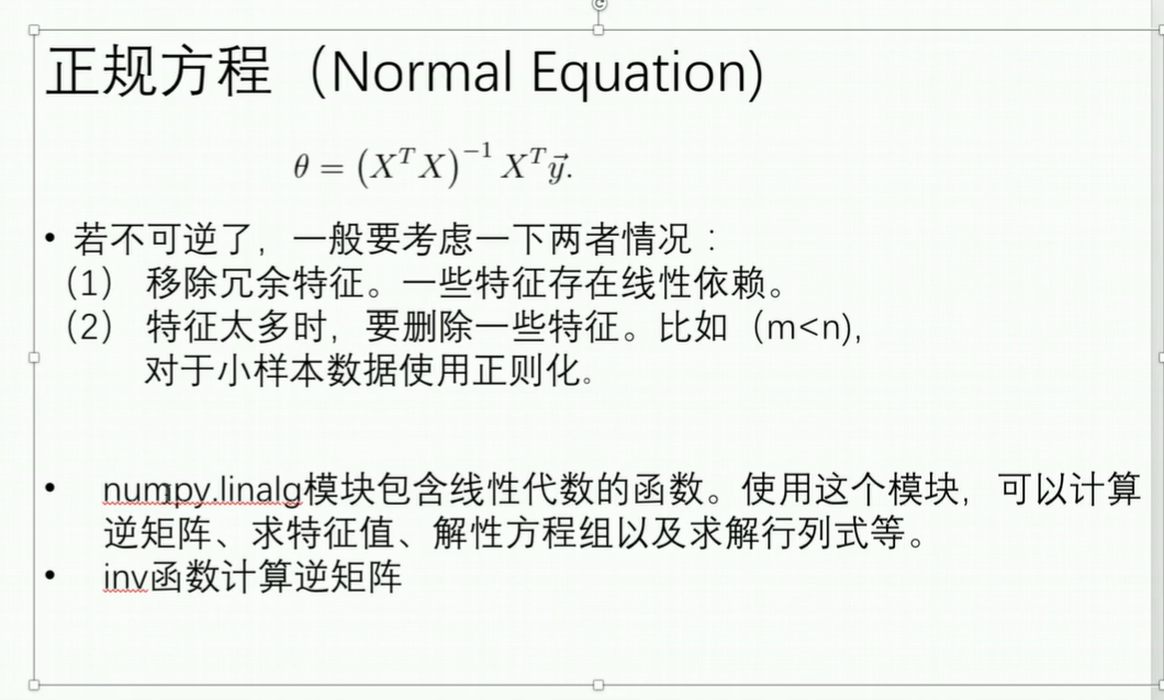
def normalEquation(X,y):
    theta=np.linalg.inv(X.T@X)@X.T@y
    return theta
theta=normalEquation(X,y)
print(theta)
x=np.linspace(y.min(),y.max(),100)
y_=theta[0,0]+theta[1,0]*x
fig,ax=plt.subplots()
ax.scatter(X[:,-1],y,label='training data')
ax.plot(x,y_,'r',label='predict')
ax.legend()
ax.set(xlabel='population',ylabel='profit')
plt.show()

可视化

问题

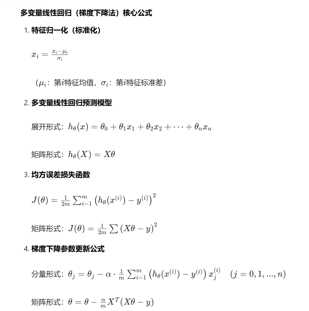
在这一部分，你将实施多变量线性回归来预测房价。假设你正在卖房子，你想知道一个好的市场价格是多少。一种方法是首先收集最近出售的房子的信息，并制作一个房价模型。文件ex1data2.txt包含俄勒冈州波特兰市房价的训练集。第一栏是房子的大小(以平方英尺为单位)，第二栏是卧室的数量，第三栏是房子的价格。

数据集

代码

import numpy as np
import pandas as pd
import matplotlib.pyplot as plt

data=pd.read_excel('D:\\小孩\\ML\\吴恩达作业\\week1线性回归\\多变量.xlsx',names=['size','bedrooms','price'])
#特征归一化
def normalize_feature(data):
    return (data-data.mean())/data.std()
data=normalize_feature(data)
data.plot.scatter(x='size',y='bedrooms',c='price')
#
data.insert(0,'ones',1)
#切片
X=data.iloc[:,0:-1]
y=data.iloc[:,-1]
X=X.values
y=y.values
y=y.reshape(46,1)

#损失函数
def costFunction(X,y,theta):
    inner=np.power(X@theta-y,2)
    return np.sum(inner)/(2*len(X))
theta=np.zeros((3,1))
cost_init=costFunction(X,y,theta)
print(cost_init)

#梯度函数
def gradientDescent(X,y,theta,alpha,iters):
    costs=[]
    for i in range(iters):
        theta=theta-(X.T@(X@theta-y))*alpha/len(X)
        cost=costFunction(X,y,theta)
        costs.append(cost)
        if i%100==0:
            print(cost)
    return theta,costs

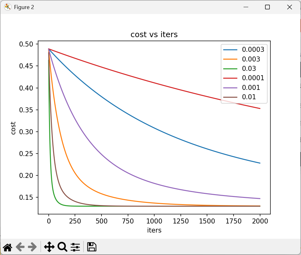
candidate_alpha=[0.0003,0.003,0.03,0.0001,0.001,0.01]
iters=2000

#损失函数图像
fig,ax=plt.subplots()
for alpha in candidate_alpha:
    _,costs=gradientDescent(X,y,theta,alpha,iters)
    ax.plot(np.arange(iters),costs,label=alpha)
    ax.legend()
ax.set(xlabel='iters',ylabel='cost',title='cost vs iters')
plt.show()

可视化

02逻辑回归

问题

你将建立一个逻辑回归模型来预测一个学生是否被大学录取。假设你是一所大学系的管理员，你想根据两次考试的成绩来决定每个申请人的录取机会。您有以前申请者的历史数据，可以用作逻辑回归的训练集。对于每个培训示例，您都有申请人在两次考试中的分数和录取决定。你的任务是建立一个分类模型，根据这两次考试的分数来估计申请人的录取概率。

数据集

代码

import numpy as np
import pandas as pd
import matplotlib.pyplot as plt

#读取数据
path='D:\\小孩\\ML\\吴恩达作业\\week2回归\\线性可分.xlsx'
data=pd.read_excel(path,names=['Exam1','Exam2','Accepted'])
data.head()#快速读取前几行（默认5）

fig,ax=plt.subplots()#创建一张画布（fig）和对应的绘图区（ax-坐标轴）
ax.scatter(data[data['Accepted']==0]['Exam1'],#x轴
           data[data['Accepted']==0]['Exam2'],#y轴
           c='r',marker='x',label='y=0')
ax.scatter(data[data['Accepted']==1]['Exam1'],
           data[data['Accepted']==1]['Exam2'],
           c='b',marker='x',label='y=1')
ax.legend()#添加图例
ax.set(xlabel='Exam 1',ylabel='Exam 2')#设置坐标轴标签
plt.show()

#初始化数据
def get_Xy(data):
    data_copy=data.copy()
    data_copy.insert(0,'ones',1)#最左边会多出一列名为ones、每行值都是 1 的列。偏移量=1
    X=data_copy.iloc[:,:-1].values# 筛选所有行、除最后一列外的所有列,转成 NumPy 数组
    y=data_copy.iloc[:,-1].values.reshape(len(data_copy),1)#选最后一列转化为Numpy一维数组，把一维数组转成列向量（二维）
    return X,y
X,y=get_Xy(data)

#代价函数
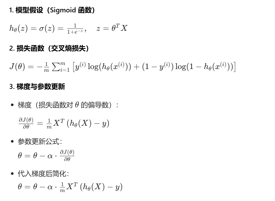
def sigmoid(z):
    return 1/(1+np.exp(-z))
def costFunction(X,y,theta):
    A=sigmoid(X.dot(theta))
    first=y*np.log(A)
    second=(1-y)*np.log(1-A)
    return -np.sum(first+second)/len(X)
theta=np.zeros((3,1))#创建一个三行一列的二维数组，所有元素为0，theta：逻辑回归的参数向量，对应公式中的θ=[θ0,θ1,θ2]
cost_init=costFunction(X,y,theta)
print("初始代价")
print(cost_init)

#梯度下降
def gradientDescent(X,y,theta,iters,alpha):
    m=len(X)
    costs=[]
    for i in range(iters):
        A=sigmoid(X@theta)
        theta=theta-(alpha/m)*X.T@(A-y)
        cost=costFunction(X,y,theta)
        costs.append(cost)
        if i%1000==0:
            print(cost)
    return costs,theta
alpha=0.004
iters=200000
costs,theta_final=gradientDescent(X,y,theta,iters,alpha)
print(theta_final)

# 预测的准确率
def predict(X,theta):
    prob=sigmoid(X@theta)
    return [1 if x>=0.5 else 0 for x in prob]
y_=np.array(predict(X,theta_final))#将预测结果从 Python 列表转换成 NumPy 一维数组
y_pre=y_.reshape(len(y_),1)#将一维的y_转换成二维列向量
acc=np.mean(y_pre==y)*100#y_pre == y：逐样本对比 "预测标签" 和 "真实标签  np.mean(...)：计算布尔数组的均值（True=1，False=0），得到 "预测正确的样本比例"；
print(f"模型预测准确率：{acc:.2f}%")  # 格式化输出

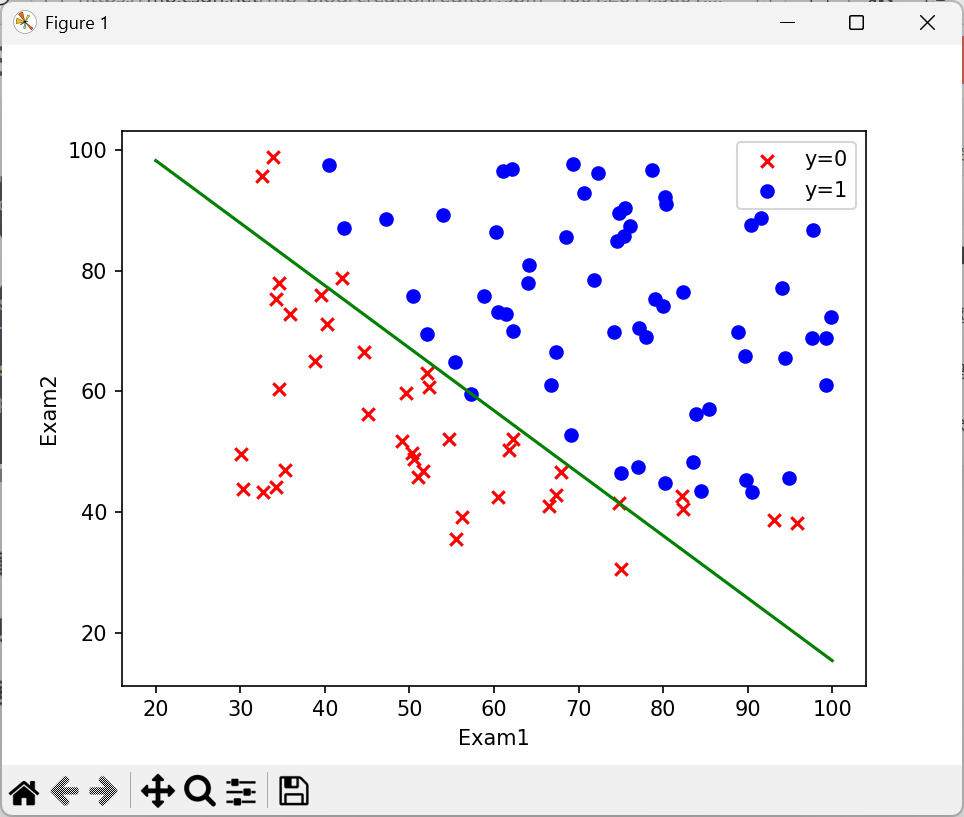
#决策边界
coef1=-theta_final[0,0]/theta_final[2,0]
coef2=-theta_final[1,0]/theta_final[2,0]
x=np.linspace(20,100,100)#np.linspace(起始值, 终止值, 点数)：在 20~100 之间生成 100 个均匀分布的数
f = coef1 + coef2 * x

#画图
fig,ax=plt.subplots()
ax.scatter(data[data['Accepted']==0]['Exam1'],data[data['Accepted']==0]['Exam2'],c='r',marker='x',label='y=0')
ax.scatter(data[data['Accepted']==1]['Exam1'],data[data['Accepted']==1]['Exam2'],c='blue',marker='o',label='y=1')
ax.legend()
ax.set(xlabel='Exam1',ylabel='Exam2')
ax.plot(x,f,c='g')
plt.show()

#预测单个学生的录取通过概率
def hfunc(theta,X):
    theta=np.array(theta)
    X=np.array(X)
    return sigmoid(X@theta)

# 示例：预测【Exam1=45，Exam2=85】的学生录取概率
pre = np.array([1, 45, 85])  # 1=偏置项，45=Exam1，85=Exam2
# 注意：theta_final是你原有代码中梯度下降得到的最优参数
the = theta_final  # 直接复用训练好的theta_final，无需转matrix
prob = hfunc(the, pre)
print(f"该同学（Exam1=45，Exam2=85）通过的概率为：{prob[0]:.4f} ({prob[0]*100:.2f}%)")

#现根据数据集把参数求出来（theta_final) 然后预测时直接带入数值 通过sigmoid函数求出录取概率

可视化

线性不可分

问题

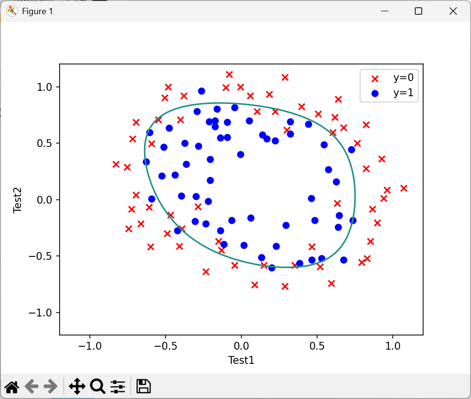
正则化逻辑回归在练习的这一部分，您将实施正则化逻辑回归来预测制造工厂的微芯片是否通过质量保证。在质量保证过程中，每个微芯片都要经过各种测试，以确保其功能正常。假设你是工厂的产品经理，你有两个不同测试的一些微芯片的测试结果。从这两个测试中，你可以决定微芯片应该被接受还是被拒绝。为了帮助您做出决定，您有一个过去微芯片的测试结果数据集，从中可以构建逻辑回归模型

数据集

代码

import numpy as np
import pandas as pd
import matplotlib.pyplot as plt

#读取数据
path='D:\\小孩\\ML\\吴恩达作业\\week2回归\\线性不可分.xlsx'
data=pd.read_excel(path,names=['Test1','Test2','Accepted'])
data.head()
fig,ax=plt.subplots()
ax.scatter(data[data['Accepted']==0]['Test1'],data[data['Accepted']==0]['Test2'],c='r',marker='x',label='y=0')
ax.scatter(data[data['Accepted']==1]['Test1'],data[data['Accepted']==1]['Test2'],c='blue',marker='o',label='y=1')
ax.legend()
ax.set(xlabel='Test1',ylabel='Test2')
plt.show()

#特征映射
def feature_mapping(x1,x2,power):
    data={}
    for i in np.arange(power+1):
        for j in np.arange(i+1):
            data['F{}{}'.format(i-j,j)]=np.power(x1,i-j)*np.power(x2,j)
    return pd.DataFrame(data)
x1=data['Test1']
x2=data['Test2']
data2=feature_mapping(x1,x2,6)
data2.head()
#构造数据集
X=data2.values
y=data.iloc[:,-1].values
y=y.reshape(len(y),1)
#损失函数
def sigmoid(z):
    return 1/(1+np.exp(-z))
def costFunction(X,y,theta,lr):
    A=sigmoid(X.dot(theta))
    first=y*np.log(A+1e-8)
    second=(1-y)*np.log(1-A)
    reg=np.sum(np.power(theta[1:],2))*(lr/(2*len(X)))
    return -np.sum(first+second)/len(X)+reg
theta=np.zeros((28,1))
lamda=1
cost_init=costFunction(X,y,theta,lamda)
print(cost_init)
#梯度下降
def gradientDescent(X,y,theta,iters,alpha,lamda):
    m=len(X)
    costs=[]
    for i in range(iters):
        reg=theta[1:]*(lamda/len(X))
        reg=np.insert(reg,0,values=0,axis=0)
        A=sigmoid(X@theta)
        theta=theta-(alpha/m)*X.T@(A-y)-reg*alpha
        cost=costFunction(X,y,theta,lamda)
        costs.append(cost)
        if i%1000==0:
            print(cost)
    return theta,costs
alpha=0.001
iters=200000
lamda=0.1
theta_final,costs=gradientDescent(X,y,theta,iters,alpha,lamda)
# 预测的准确率
def predict(X,theta):
    prob=sigmoid(X@theta)
    return [1 if x>=0.5 else 0 for x in prob]
y_=np.array(predict(X,theta_final))#将预测结果从 Python 列表转换成 NumPy 一维数组
y_pre=y_.reshape(len(y_),1)#将一维的y_转换成二维列向量
acc=np.mean(y_pre==y)*100#y_pre == y：逐样本对比 "预测标签" 和 "真实标签  np.mean(...)：计算布尔数组的均值（True=1，False=0），得到 "预测正确的样本比例"；
print(f"模型预测准确率：{acc:.2f}%")  # 格式化输出

# 1. 生成x轴的等距数值（范围-1.2到1.2，共200个点）
x = np.linspace(-1.2, 1.2, 200)
# 2. 生成二维网格（xx是x轴网格，yy是y轴网格，形状都是(200,200)）
xx, yy = np.meshgrid(x, x)
# 3. 对网格点做6次特征映射（和训练时一致）
# ravel()：把二维网格展平为一维数组（200*200=40000个点）
z = feature_mapping(xx.ravel(), yy.ravel(), 6).values
# 4. 计算每个网格点的线性得分（z @ theta_final 等价于 X*θ）
zz = z @ theta_final
# 5. 把一维得分转回二维网格形状（200,200），用于绘图
zz = zz.reshape(xx.shape)

fig,ax=plt.subplots()
ax.scatter(data[data['Accepted']==0]['Test1'],data[data['Accepted']==0]['Test2'],c='r',marker='x',label='y=0')
ax.scatter(data[data['Accepted']==1]['Test1'],data[data['Accepted']==1]['Test2'],c='blue',marker='o',label='y=1')
ax.legend()
ax.set(xlabel='Test1',ylabel='Test2')
plt.contour(xx,yy,zz,0)
plt.show()

可视化

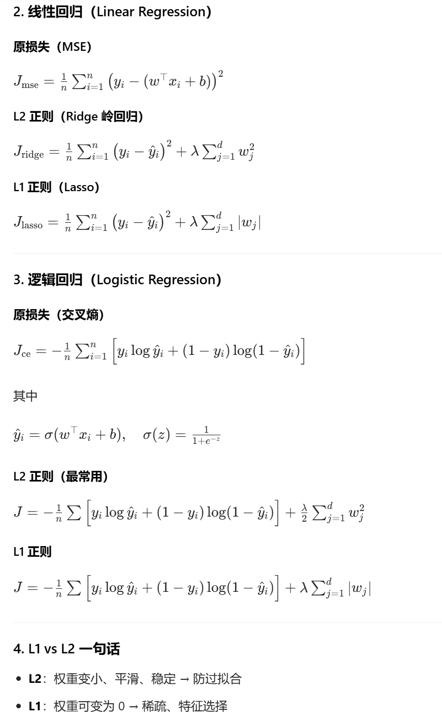
正则化

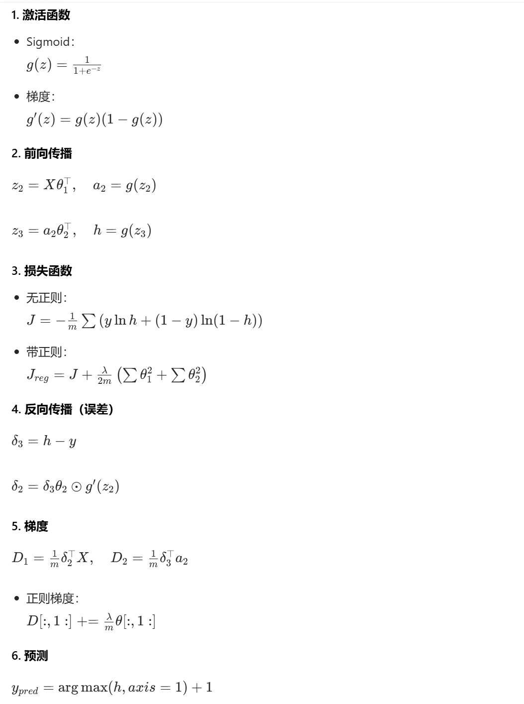
03神经网络

题目

这部分，你需要实现一个可以识别手写数字的神经网络。神经网络可以表示一些非线性复杂的模型。权重已经预先训练好，你的目标是在现有权重基础上，实现前馈神经网络。

若已给定神经网络中的theta矩阵（需要用反向传播算法得出），实现前馈神经网络，理解神经网络的作用。

题目已给出a(1)为第一层输入层数据，有400个神经元代表每个数字的图像（不加偏置值）；

a(2)为隐藏层，有25个神经元（不加偏置值）；

a(3)为输出层'，又10个神经元，以10个（0/1）值的向量表示；

theta1为第一层到第二层的参数矩阵（25，401）；

theta2为第二层到第三层的参数矩阵（10，26）。

代码

import numpy as np
import scipy.io as sio
import matplotlib.pyplot as plt

data=sio.loadmat('D:\\小孩\\ML\\吴恩达作业\\ML_NG\\03-neural network\\ex3data1.mat')

raw_X = data['X']
raw_y = data['y']
#随机打印一个图片
def plot_an_image(X):
    pick_one=np.random.randint(5000)
    image=X[pick_one,:]
    fig,ax=plt.subplots(figsize=(1,1))
    ax.imshow(image.reshape(20,20).T,cmap='gray_r')
    plt.xticks([])#删掉刻度
    plt.yticks([])
plot_an_image(raw_X)
plt.show()
#打印一百张
def plot_100_image(X):
    sample_index=np.random.choice(len(X),100)
    images=X[sample_index,:]
    print(images.shape)
    fig,ax=plt.subplots(ncols=10,nrows=10,figsize=(8,8),sharex=True,sharey=True)
    for i in range(10):
        for j in range(10):
            ax[i,j].imshow(images[10*i+j].reshape(20,20).T,cmap='gray_r')
    plt.xticks([])  # 删掉刻度
    plt.yticks([])
plot_100_image(raw_X)
plt.show()
#
def sigmoid(z):
    return 1/(1+np.exp(-z))
def costFunction(theta,X,y,lamda):
    A=sigmoid(X.dot(theta))
    first=y*np.log(A+1e-8)
    second=(1-y)*np.log(1-A)
    reg=theta[1:]@theta[1:]*(lamda/(2*len(X)))#一维
    return -np.sum(first+second)/len(X)+reg
def gradient_reg(theta,X,y,lamda):
    reg=theta[1:]*(lamda/len(X))
    reg=np.insert(reg,0,values=0,axis=0)
    first=(X.T@(sigmoid(X@theta)-y))/len(X)
    return first+reg
X=np.insert(raw_X,0,values=1,axis=1)
y=raw_y.flatten()

from scipy.optimize import minimize
def one_vs_all(X,y,lamda,K):
    n=X.shape[1]
    theta_all=np.zeros((K,n))
    for i in range(1,K+1):
        theta_i=np.zeros(n,)
        res=minimize(fun=costFunction,
                     x0=theta_i,
                     args=(X,y==i,lamda),
                     method='TNC',
                     jac=gradient_reg)
        theta_all[i-1,:]=res.x
    return theta_all
lamda=1
K=10
theta_final=one_vs_all(X,y,lamda,K)
print(theta_final)
def predict(X,theta_final):
    h=sigmoid(X@theta_final.T)
    h_argmax=np.argmax(h,axis=1)
    return h_argmax+1
y_pred=predict(X,theta_final)
acc=np.mean(y==y_pred)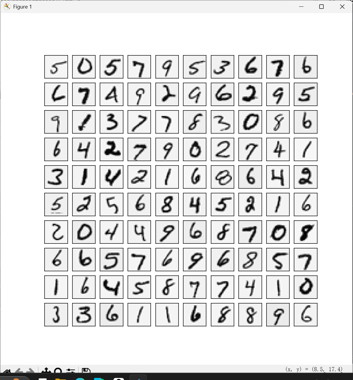

前向传播

import numpy as np
import scipy.io as sio
import matplotlib.pyplot as plt

data=sio.loadmat('D:\\小孩\\ML\\吴恩达作业\\ML_NG\\03-neural network\\ex3data1.mat')

raw_X = data['X']
raw_y = data['y']
X=np.insert(raw_X,0,values=1,axis=1)
y=raw_y.flatten()
theta=sio.loadmat('D:\\小孩\\ML\\吴恩达作业\\ML_NG\\03-neural network\\ex3weights.mat')
theta.keys()
theta1=theta['Theta1']
theta2=theta['Theta2']
#
def sigmoid(z):
    return 1/(1+np.exp(-z))
a1=X
z2=X@theta1.T
a2=sigmoid(z2)
a2=np.insert(a2,0,values=1,axis=1)
z3=a2@theta2.T
a3=sigmoid(z3)
y_pred=np.argmax(a3,axis=1)
y_pred=y_pred+1
acc=np.mean(y==y_pred)
print(acc)

反向传播

import numpy as np
import scipy.io as sio
import matplotlib.pyplot as plt
data=sio.loadmat('D:\\小孩\\ML\\吴恩达作业\\ML_NG\\04-neural network(bp)\\ex4data1.mat')
raw_X=data['X']
raw_y=data['y']
X=np.insert(raw_X,0,values=1,axis=1)
#one-hot编码:把「数字标签」变成「神经网络能懂的二进制向量」
def one_hot_encoder(raw_y):
    result=[]
    for i in raw_y:
        y_temp=np.zeros(10)
        y_temp[i-1]=1
        result.append(y_temp)
    return np.array(result)
y=one_hot_encoder(raw_y)
theta_data=sio.loadmat('D:\\小孩\\ML\\吴恩达作业\\ML_NG\\04-neural network(bp)\\ex4weights.mat')
theta1,theta2=theta_data['Theta1'],theta_data['Theta2']

#序列化权重参数
#序列化的目的：适配优化函数minimize的格式要求（只认一维数组），让它能调参
def serialize(a,b):
    #a.flatten()把多维矩阵 "拍扁" 成一维
    return np.append(a.flatten(),b.flatten())
theta_serialize=serialize(theta1,theta2)

#解序列化权重参数
#解序列化的目的：适配神经网络的计算要求（只认矩阵），让调完的参数能用来做前向 / 反向传播
def deserialize(theta_serialize):
    theta1=theta_serialize[:25*401].reshape(25,401)
    theta2=theta_serialize[25*401:].reshape(10,26)
    return theta1,theta2
theta1,theta2=deserialize(theta_serialize)

#前向传播
def sigmoid(z):
    return 1/(1+np.exp(-z))
def feed_forward(theta_serialize,X):
    theta1,theta2=deserialize(theta_serialize)
    a1=X
    z2=a1@theta1.T
    a2=sigmoid(z2)
    a2=np.insert(a2,0,values=1,axis=1)
    z3=a2@theta2.T
    h=sigmoid(z3)
    return a1,z2,a2,z3,h

#损失函数
#5-1不带正则化的损失函数
def cost(theta_serialize,X,y):
    a1,z2,a2,z3,h=feed_forward(theta_serialize,X)
    J=-np.sum(y*np.log(h)+(1-y)*np.log(1-h))/len(X)
    return J
#5-2带正则化的损失函数
def reg_cost(theta_serialize,X,y,lamda):
    sum1=np.sum(np.power(theta1[:,1:],2))
    sum2=np.sum(np.power(theta2[:,1:],2))
    reg=(sum1+sum2)*lamda/(2*len(X))
    return reg+cost(theta_serialize,X,y)
lamda=1

#反向传播
#无正则化的梯度
def sigmoid_gradient(z):
    return sigmoid(z)*(1-sigmoid(z))
def gradient(theta_serialize,X,y):
    theta1,theta2=deserialize(theta_serialize)
    a1,z2,a2,z3,h=feed_forward(theta_serialize,X)
    d3=h-y
    d2=d3@theta2[:,1:]*sigmoid_gradient(z2)
    D2=(d3.T@a2)/len(X)
    D1=(d2.T@a1)/len(X)
    return serialize(D1,D2)
#带正则化的梯度
def reg_gradient(theta_serialize,X,y,lamda):
    D=gradient(theta_serialize,X,y)
    D1,D2=deserialize(D)
    theta1,theta2=deserialize(theta_serialize)
    D1[:,1:]=D1[:,1:]+theta1[:,1:]*lamda/len(X)
    D2[:,1:]=D2[:,1:]+theta2[:,1:]*lamda/len(X)
    return serialize(D1,D2)



#为什么不在序列化之前就向前向后传播呢，传播完了再序列化进行优化
#优化函数要 "反复调用传播函数"，而调用的前提是 "参数是一维数组"
#优化(正则化）(限制过拟合）
from scipy.optimize import minimize
def nn_training(X,y):
    init_theta=np.random.uniform(-0.5,0.5,10285)
    res=minimize(fun=reg_cost,
                 x0=init_theta,
                 args=(X,y,lamda),
                 method='TNC',
                 jac=reg_gradient,
                 options={'maxfun':300}
                 )
    return res
lamda=10
res=nn_training(X,y)
raw_y=data['y'].reshape(5000,)
_,_,_,_,h=feed_forward(res.x,X)
y_pred=np.argmax(h,axis=1)+1
acc=np.mean(y_pred==raw_y)

#可视化隐藏层
def plot_hidden_layer(theta):
    theta1,_=deserialize(theta)
    hidden_layer=theta1[:,1:]
    fig,ax=plt.subplots(ncols=5,nrows=5,figsize=(8,8),sharex=True,sharey=True)
    for i in range(5):
        for j in range(5):
            ax[i,j].imshow(hidden_layer[i*5+j].reshape(20,20).T,cmap='gray_r')
    plt.xticks([])
    plt.yticks([])
    plt.show()
plot_hidden_layer(res.x)