一维概率分布可视化实践:基于 Python 的理论曲线与样本图对照
概率分布是概率论、数理统计、数据分析与机器学习中的基础内容。学习分布时,除了掌握定义和公式,更重要的是理解分布的形状、参数变化带来的影响,以及随机样本与理论分布之间的关系。
本文基于一套统一的绘图函数,对常见连续型分布和离散型分布进行可视化展示。每个分布都包含两部分内容:一部分是理论图像,用于展示 PDF / PMF 和 CDF 的形状;另一部分是随机样本图,用于对比样本频数与理论分布之间的关系。通过这种方式,可以更直观地理解不同分布的特征,以及样本量增大时经验分布向理论分布逼近的过程。
0. 绘图函数封装(通用)
在具体展示各类分布之前,先对绘图逻辑进行统一封装。这样做的主要目的,是避免在每个分布小节中重复处理坐标范围、图例、字体、样本频数与理论曲线叠加等细节,使后续示例更聚焦于分布本身。
python
import numpy as np
import matplotlib.pyplot as plt
import seaborn as sns
from matplotlib.font_manager import FontProperties

# =========================
# 全局字体设置
# =========================
# 解决坐标轴负号显示为方块的问题
plt.rcParams['axes.unicode_minus'] = False
# 数学公式字体风格设置为 stix,便于与 Times New Roman 风格协调
plt.rcParams['mathtext.fontset'] = 'stix'
# 全局默认字体族设置为衬线字体
plt.rcParams['font.family'] = 'serif'

# 英文 / 数学 / 数字使用 Times New Roman
font_en = FontProperties(family='Times New Roman')
# 中文使用宋体
font_cn = FontProperties(family='SimSun')
# 中英混排时,同时指定英文和中文字体
font_mix = FontProperties(family=['Times New Roman', 'SimSun'])

# 不同样本规模,用于观察样本量增大时,经验分布如何逼近理论分布
SIZES = [100, 10000, 1000000]


# =========================
# 工具函数
# =========================
def set_count_formatter(ax):
    """
    给 y 轴设置千分位格式,例如 10000 -> 10,000
    主要用于频数坐标轴显示,提升可读性
    """
    formatter = plt.FuncFormatter(lambda x, _: '{:,.0f}'.format(x))
    ax.yaxis.set_major_formatter(formatter)


def get_continuous_plot_range(
    dist,
    data=None,
    q_low=0.005,
    q_high=0.995,
    hard_clip=None,
    fixed_range=None
):
    """
    计算连续型分布绘图时的横轴范围。

    优先级说明:
    1. 如果传入 fixed_range,则直接使用固定范围;
    2. 否则尝试结合理论分布分位点和样本分位点自动确定范围;
    3. 如仍无法确定,则退化为样本最小/最大值,或默认 [-5, 5]。

    参数:
    - dist: scipy.stats 风格的连续分布对象,需支持 ppf
    - data: 样本数据,可选
    - q_low, q_high: 用于截取中间主体区间的低/高分位点
    - hard_clip: 强制裁剪范围,例如 (0, None) 表示下界不小于 0
    - fixed_range: 直接指定绘图区间 (low, high)

    返回:
    - low, high: 绘图横轴范围
    """
    # 如果用户明确指定了范围,则直接使用
    if fixed_range is not None:
        low, high = fixed_range
    else:
        # 理论分布对应的分位点范围
        theory_low, theory_high = None, None
        try:
            theory_low = dist.ppf(q_low)
            theory_high = dist.ppf(q_high)
        except Exception:
            # 某些分布可能不支持 ppf,或返回异常值
            pass

        # 样本数据对应的分位点范围
        data_low, data_high = None, None
        if data is not None and len(data) > 0:
            data_low = np.quantile(data, q_low)
            data_high = np.quantile(data, q_high)

        # 只保留有效且有限的下界/上界
        lows = [v for v in [theory_low, data_low] if v is not None and np.isfinite(v)]
        highs = [v for v in [theory_high, data_high] if v is not None and np.isfinite(v)]

        # 如果理论和样本分位点都无效,则退化处理
        if len(lows) == 0 or len(highs) == 0:
            if data is not None and len(data) > 0:
                # 有样本时直接用样本最小值和最大值
                low, high = np.min(data), np.max(data)
            else:
                # 没有样本也没有理论范围时,给一个默认区间
                low, high = -5, 5
        else:
            # 用理论与样本中更保守的范围,尽量覆盖主要分布区域
            low, high = min(lows), max(highs)

        # 给范围留出 5% 的边距,避免图形顶边或贴边
        span = high - low
        if span <= 0:
            span = 1.0
        low -= 0.05 * span
        high += 0.05 * span

    # 如果设置了硬裁剪范围,则进一步限制上下界
    if hard_clip is not None:
        if hard_clip[0] is not None:
            low = max(low, hard_clip[0])
        if hard_clip[1] is not None:
            high = min(high, hard_clip[1])

    # 最终再做一次安全检查,确保 low/high 有效且 low < high
    if not np.isfinite(low) or not np.isfinite(high) or low >= high:
        low, high = -5, 5

    return low, high


def get_discrete_support_by_cdf(dist, start=0, threshold=0.995, max_k=1000):
    """
    根据离散分布的 CDF 自动确定绘图支持集范围。

    思路:
    从 start 开始枚举到 max_k,找到最小的 k,使得 CDF(k) >= threshold,
    然后返回 [start, k] 这段整数支持集。

    参数:
    - dist: scipy.stats 风格的离散分布对象,需支持 cdf
    - start: 起始取值
    - threshold: CDF 截断阈值,例如 0.995 表示覆盖 99.5% 概率质量
    - max_k: 最大搜索上限,防止无限增长

    返回:
    - xs[:idx + 1]: 需要绘制的整数取值范围
    """
    xs = np.arange(start, max_k + 1)
    cdf_vals = dist.cdf(xs)
    idx = np.searchsorted(cdf_vals, threshold)

    # 若直到 max_k 仍未达到阈值,则返回整个搜索范围
    if idx >= len(xs):
        return xs
    return xs[:idx + 1]


# =========================
# 理论图:连续型 PDF + CDF
# =========================
def plot_continuous_theory(
    title,
    dist_list,
    labels,
    x_range,
    xlabel='x',
    pdf_ylabel='PDF',
    cdf_ylabel='CDF',
    title_suffix=':理论 PDF 与 CDF'
):
    """
    绘制连续型分布的理论 PDF 和 CDF 曲线。

    参数:
    - title: 图标题主体
    - dist_list: 分布对象列表
    - labels: 每个分布对应的图例标签
    - x_range: 横轴范围 (xmin, xmax)
    - xlabel: 横轴标签
    - pdf_ylabel: 左图纵轴标签
    - cdf_ylabel: 右图纵轴标签
    - title_suffix: 图总标题后缀
    """
    # 在给定区间内均匀取点,用于绘制连续曲线
    x = np.linspace(x_range[0], x_range[1], 1000)

    # 创建 1 行 2 列子图:左边 PDF,右边 CDF
    fig, axs = plt.subplots(1, 2, figsize=(12, 4))

    # -------- 左图:PDF --------
    ax1 = axs[0]
    for dist, label in zip(dist_list, labels):
        ax1.plot(x, dist.pdf(x), label=label)
    ax1.set_xlim(x_range[0], x_range[1])
    ax1.set_xlabel(xlabel, fontsize=15, fontproperties=font_en)
    ax1.set_ylabel(pdf_ylabel, fontsize=15, fontproperties=font_en)
    ax1.legend(prop=font_mix)
    ax1.grid(True)

    # -------- 右图:CDF --------
    ax2 = axs[1]
    for dist, label in zip(dist_list, labels):
        ax2.plot(x, dist.cdf(x), label=label)
    ax2.set_xlim(x_range[0], x_range[1])
    ax2.set_xlabel(xlabel, fontsize=15, fontproperties=font_en)
    ax2.set_ylabel(cdf_ylabel, fontsize=15, fontproperties=font_en)
    ax2.legend(prop=font_mix)
    ax2.grid(True)

    # 设置总标题并自动调整布局
    plt.suptitle(title + title_suffix, fontsize=16, fontproperties=font_mix)
    plt.tight_layout()
    plt.show()


# =========================
# 理论图:离散型 PMF + CDF
# =========================
def plot_discrete_theory(
    title,
    dist_list,
    labels,
    x_values,
    xlabel='x',
    pmf_ylabel='PMF',
    cdf_ylabel='CDF',
    title_suffix=':理论 PMF 与 CDF'
):
    """
    绘制离散型分布的理论 PMF 和 CDF 图像。

    参数:
    - title: 图标题主体
    - dist_list: 分布对象列表
    - labels: 每个分布的标签
    - x_values: 离散取值点
    - xlabel: 横轴标签
    - pmf_ylabel: 左图纵轴标签
    - cdf_ylabel: 右图纵轴标签
    - title_suffix: 图总标题后缀
    """
    fig, axs = plt.subplots(1, 2, figsize=(12, 4))

    # -------- 左图:PMF --------
    ax1 = axs[0]
    for dist, label in zip(dist_list, labels):
        # stem 图适合表现离散分布的点质量函数
        markerline, stemlines, baseline = ax1.stem(
            x_values, dist.pmf(x_values), linefmt='-', markerfmt='o', basefmt=' '
        )
        markerline.set_label(label)
    ax1.set_xlabel(xlabel, fontsize=15, fontproperties=font_en)
    ax1.set_ylabel(pmf_ylabel, fontsize=15, fontproperties=font_en)
    ax1.legend(prop=font_mix)
    ax1.grid(True)

    # -------- 右图:CDF --------
    ax2 = axs[1]
    for dist, label in zip(dist_list, labels):
        # 离散型分布函数用阶梯图更符合其本质
        ax2.step(x_values, dist.cdf(x_values), where='post', label=label)
    ax2.set_xlabel(xlabel, fontsize=15, fontproperties=font_en)
    ax2.set_ylabel(cdf_ylabel, fontsize=15, fontproperties=font_en)
    ax2.legend(prop=font_mix)
    ax2.grid(True)

    plt.suptitle(title + title_suffix, fontsize=16, fontproperties=font_mix)
    plt.tight_layout()
    plt.show()


# =========================
# 随机样本图:连续型
# =========================
def plot_continuous_samples(
    title,
    sampler,
    dist,
    bins=40,
    sizes=SIZES,
    q_low=0.005,
    q_high=0.995,
    hard_clip=None,
    fixed_range=None,
    xlabel='数值',
    ylabel_left='频数',
    ylabel_right='密度'
):
    """
    绘制连续型随机样本的直方图,并叠加理论 PDF。

    设计思路:
    - 横向展示多个样本规模(默认 100、10000、1000000)
    - 左 y 轴显示频数
    - 右 y 轴显示密度
    - 将理论 PDF 按"频数尺度"缩放后叠加到直方图上,便于直接比较

    参数:
    - title: 图标题主体
    - sampler: 抽样函数,输入样本量 size,输出样本数组
    - dist: 理论分布对象,需支持 pdf
    - bins: 直方图箱数
    - sizes: 样本规模列表
    - q_low, q_high: 自动确定横轴范围时使用的分位点
    - hard_clip: 强制裁剪横轴范围
    - fixed_range: 固定横轴范围
    - xlabel: 横轴标签
    - ylabel_left: 左纵轴标签(频数)
    - ylabel_right: 右纵轴标签(密度)
    """
    # 创建 1 行 3 列子图,共享 x 轴范围
    fig, axs = plt.subplots(1, 3, figsize=(22, 6), sharex=True)

    for ax, size in zip(axs, sizes):
        # 生成指定样本量的数据
        data = sampler(size)

        # 根据理论分布和样本数据自动确定绘图区间
        x_min, x_max = get_continuous_plot_range(
            dist=dist,
            data=data,
            q_low=q_low,
            q_high=q_high,
            hard_clip=hard_clip,
            fixed_range=fixed_range
        )

        # 构造直方图箱边界
        bins_arr = np.linspace(x_min, x_max, bins + 1)
        # 用于绘制理论 PDF 曲线的稠密横坐标
        x = np.linspace(x_min, x_max, 1000)
        # 单个箱子的宽度
        bin_width = bins_arr[1] - bins_arr[0]

        # 绘制样本直方图(频数形式)
        sns.histplot(
            data=data,
            bins=bins_arr,
            color='skyblue',
            edgecolor='black',
            ax=ax
        )

        # 将理论 PDF 转换为"期望频数"尺度:
        # 密度 × 样本量 × 箱宽 = 每个箱子的理论期望频数
        y = dist.pdf(x) * len(data) * bin_width
        ax.plot(x, y, 'r--', linewidth=2, label='Theory PDF')

        ax.set_xlim(x_min, x_max)
        ax.set_title(f'N = {"{:,}".format(len(data))}', fontsize=14, fontproperties=font_en)
        ax.set_ylabel(ylabel_left, fontsize=15, fontproperties=font_cn)
        ax.grid(True)
        ax.legend(prop=font_en)

        # 创建右侧 y 轴,用于显示密度刻度
        ax2 = ax.twinx()
        ylim1 = ax.get_ylim()

        # 左轴频数 -> 右轴密度 的换算关系:
        # 密度 = 频数 / (样本量 × 箱宽)
        ax2.set_ylim((ylim1[0] / len(data) / bin_width, ylim1[1] / len(data) / bin_width))
        ax2.set_ylabel(ylabel_right, fontsize=15, fontproperties=font_cn)

        # 设置刻度字体大小
        ax.tick_params(axis='both', labelsize=14)
        ax2.tick_params(axis='both', labelsize=14)

        # 左轴频数采用千分位格式
        set_count_formatter(ax)

    # 设置总标题和整个图的公共 x 轴标题
    fig.suptitle(title + ':样本与理论密度对比', fontsize=20, fontproperties=font_mix)
    fig.text(0.5, 0, xlabel, ha='center', fontsize=12, fontproperties=font_cn)
    plt.tight_layout()
    plt.show()


# =========================
# 随机样本图:离散型
# =========================
def plot_discrete_samples(
    title,
    sampler,
    dist,
    sizes=SIZES,
    x_values=None,
    cdf_threshold=0.995,
    start=0,
    xlabel='数值',
    ylabel_left='频数',
    ylabel_right='概率'
):
    """
    绘制离散型随机样本的频数图,并叠加理论 PMF。

    设计思路:
    - 如果未指定 x_values,则自动根据 CDF 截断得到支持集
    - 左 y 轴显示频数
    - 右 y 轴显示概率
    - 理论 PMF 按样本量放缩后叠加到样本频数图上

    参数:
    - title: 图标题主体
    - sampler: 抽样函数
    - dist: 理论离散分布对象,需支持 pmf / cdf
    - sizes: 样本规模列表
    - x_values: 指定离散支持集
    - cdf_threshold: 自动确定支持集时的累计概率阈值
    - start: 支持集起点
    - xlabel: 横轴标签
    - ylabel_left: 左纵轴标签(频数)
    - ylabel_right: 右纵轴标签(概率)
    """
    fig, axs = plt.subplots(1, 3, figsize=(22, 6), sharex=True)

    # 如果没有给定离散支持集,则自动根据 CDF 计算一个足够覆盖主要概率质量的范围
    if x_values is None:
        x_values = get_discrete_support_by_cdf(
            dist=dist,
            start=start,
            threshold=cdf_threshold,
            max_k=1000
        )

    x_min, x_max = x_values.min(), x_values.max()

    for ax, size in zip(axs, sizes):
        # 生成样本
        data = sampler(size)

        # 为了让整数值落在箱体中心,构造半整数边界
        bins = np.arange(x_min - 0.5, x_max + 1.5, 1)

        # 绘制离散直方图
        sns.histplot(
            data=data,
            bins=bins,
            color='skyblue',
            edgecolor='black',
            ax=ax,
            discrete=True
        )

        # 将理论 PMF 放缩到频数尺度:
        # 概率 × 样本量 = 理论期望频数
        pmf = dist.pmf(x_values) * len(data)
        ax.plot(x_values, pmf, 'r--', linewidth=2, marker='o', markersize=4, label='Theory PMF')

        ax.set_xlim(x_min - 0.5, x_max + 0.5)
        ax.set_title(f'N = {"{:,}".format(len(data))}', fontsize=14, fontproperties=font_en)
        ax.set_ylabel(ylabel_left, fontsize=15, fontproperties=font_cn)
        ax.grid(True)
        ax.legend(prop=font_en)

        # 创建右侧 y 轴,用于显示概率尺度
        ax2 = ax.twinx()
        ylim1 = ax.get_ylim()

        # 左轴频数 -> 右轴概率 的换算关系:
        # 概率 = 频数 / 样本量
        ax2.set_ylim((ylim1[0] / len(data), ylim1[1] / len(data)))
        ax2.set_ylabel(ylabel_right, fontsize=15, fontproperties=font_cn)

        # 设置刻度字体大小
        ax.tick_params(axis='both', labelsize=14)
        ax2.tick_params(axis='both', labelsize=14)

        # 左轴频数采用千分位显示
        set_count_formatter(ax)

    # 设置总标题和全图公共 x 轴标题
    fig.suptitle(title + ':样本与理论概率对比', fontsize=20, fontproperties=font_mix)
    fig.text(0.5, 0, xlabel, ha='center', fontsize=12, fontproperties=font_cn)
    plt.tight_layout()
    plt.show()
这里有一个容易被忽略但非常重要的细节:在连续型分布的样本图中,叠加的理论曲线并不是简单地画 dist.pdf(x),而是乘上了样本量和组距,也就是:
python
y = dist.pdf(x) * len(data) * bin_width原因在于直方图默认展示的是频数,而 PDF 展示的是概率密度,两者量纲不同,不能直接放在同一纵轴上比较。只有经过这一步缩放之后,理论曲线才会和频数直方图落在同一尺度下。同样地,在离散型分布中,PMF 会乘以样本量,从而转换为"理论期望频数",便于与样本频数图直接对照。
1. 连续性概率分布
连续型分布通常通过概率密度函数(PDF)和累积分布函数(CDF)进行描述。本文选择若干常见分布进行展示,重点观察它们的形状特征、参数变化以及样本与理论之间的对应关系。
1.1 正态分布 (Normal)
正态分布是概率统计中最经典、最重要的分布之一。在实际问题中,测量误差、自然波动、中心极限定理下的样本均值,都会与正态分布产生密切联系。它的密度函数为:
f(x∣μ,σ2)=12πσ2exp(−(x−μ)22σ2) f(x|\mu,\sigma^2)=\frac{1}{\sqrt{2\pi\sigma^2}}\exp\Big(-\frac{(x-\mu)^2}{2\sigma^2}\Big) f(x∣μ,σ2)=2πσ2 1exp(−2σ2(x−μ)2)
它的密度函数由均值 μ\muμ 和方差 σ2\sigma^2σ2 决定,其中 μ\muμ 控制分布中心的位置,σ2\sigma^2σ2 控制分布的离散程度。均值不变时,方差越大,曲线越平缓;方差越小,曲线越尖锐。
python
from scipy.stats import norm

parameters = [(0, 0.2), (0, 1.0), (0, 5.0), (-2, 0.5)]
normal_dists = [norm(loc=mu, scale=np.sqrt(sigma_sq)) for mu, sigma_sq in parameters]
normal_labels = [r'$\mu$=' + f'{mu}, ' + r'$\sigma^2$=' + f'{sigma_sq}' for mu, sigma_sq in parameters]

plot_continuous_theory(
    title='正态分布 Normal',
    dist_list=normal_dists,
    labels=normal_labels,
    x_range=(-5.5, 5.5),
    xlabel='x',
    pdf_ylabel=r'$\phi_{\mu,\sigma^2}(x)$',
    cdf_ylabel=r'$\Phi_{\mu,\sigma^2}(x)$'
)
plot_continuous_samples(
    title='正态分布 Normal(0,1)',
    sampler=lambda n: np.random.normal(0, 1, n),
    dist=norm(0, 1),
    bins=40,
    fixed_range=(-4, 4)
)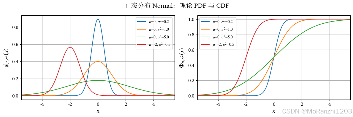
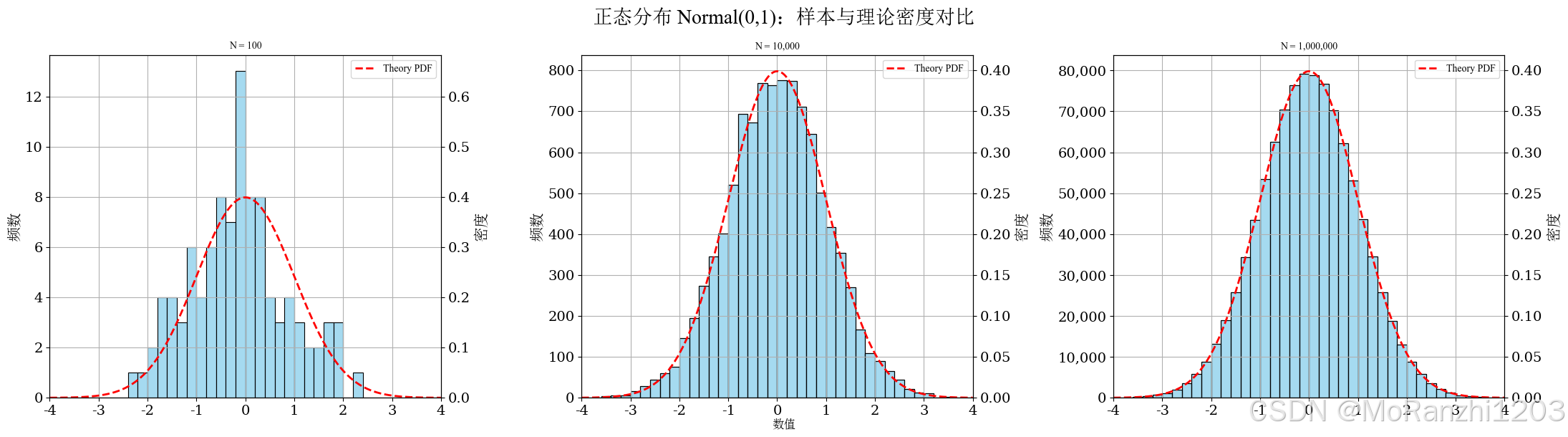
在图像上,均值变化会引起曲线整体平移,方差变化会改变曲线的宽窄和峰值高度。方差越大,曲线越平缓;方差越小,曲线越集中。样本图中可以看到,随着样本量增加,直方图逐渐接近理论曲线,这也是经验分布逼近理论分布的直观体现。
1.2 连续均匀分布 (Uniform)
连续均匀分布表示随机变量在区间 a,ba,ba,b 上每一个位置出现的可能性完全相同。它的密度函数写作:
f(x∣a,b)=1b−a,x∈a,b f(x|a,b) = \frac{1}{b-a}, \quad x \in a,b f(x∣a,b)=b−a1,x∈a,b
这类分布在随机模拟中非常常见,也是很多随机数生成方法的基础。它的形状非常直观:在定义区间内是一条水平直线,区间之外则为 0。
python
from scipy.stats import uniform

uniform_dists = [uniform(loc=-4, scale=8), uniform(loc=-2, scale=4), uniform(loc=0, scale=2)]
uniform_labels = [r'$U(-4,4)$', r'$U(-2,2)$', r'$U(0,2)$']

plot_continuous_theory(
    title='连续均匀分布 Uniform',
    dist_list=uniform_dists,
    labels=uniform_labels,
    x_range=(-5, 5)
)
plot_continuous_samples(
    title='连续均匀分布 Uniform(-4,4)',
    sampler=lambda n: np.random.uniform(-4, 4, n),
    dist=uniform(loc=-4, scale=8),
    bins=40,
    fixed_range=(-4, 4)
)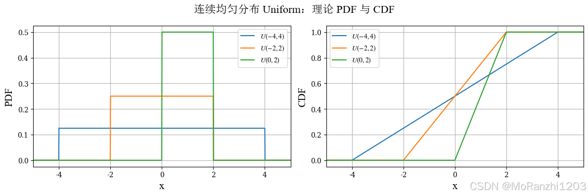
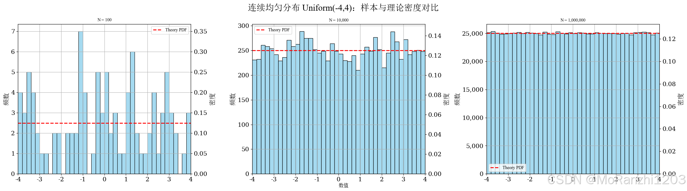
均匀分布的参数直接决定支持区间的位置和长度。区间越宽,密度值越低;区间越窄,密度值越高。它常用于随机模拟,也常作为其他采样方法的基础分布。
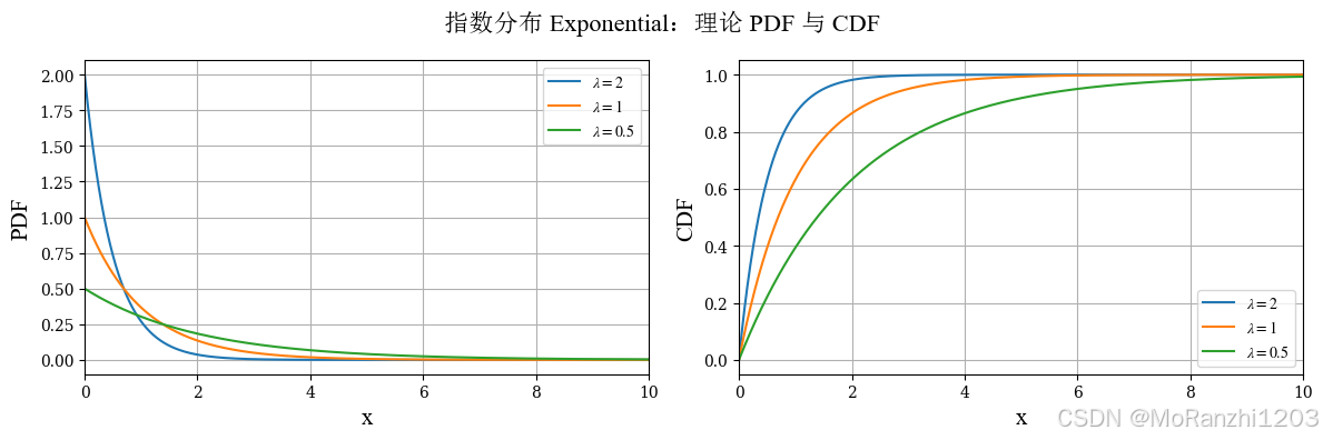
1.3 指数分布 (Exponential)
指数分布通常用于描述等待时间问题,例如事件发生的间隔时间、系统寿命等。它定义在非负实数范围上,密度函数随自变量增大而单调衰减。它的概率密度函数为:
f(x∣λ)=λe−λx,x≥0 f(x|\lambda) = \lambda e^{-\lambda x}, \quad x \ge 0 f(x∣λ)=λe−λx,x≥0
指数分布的参数 λ\lambdaλ 控制衰减速度。λ\lambdaλ 越大,分布越集中在靠近零的位置;λ\lambdaλ 越小,尾部越长。指数分布的一个重要性质是无记忆性,这也是它在随机过程和排队论中广泛使用的原因。
python
from scipy.stats import expon
expon_dists = [expon(scale=0.5), expon(scale=1), expon(scale=2)]
expon_labels = [r'$\lambda=2$', r'$\lambda=1$', r'$\lambda=0.5$']
plot_continuous_theory(
title='指数分布 Exponential',
dist_list=expon_dists,
labels=expon_labels,
x_range=(0, 10)
)
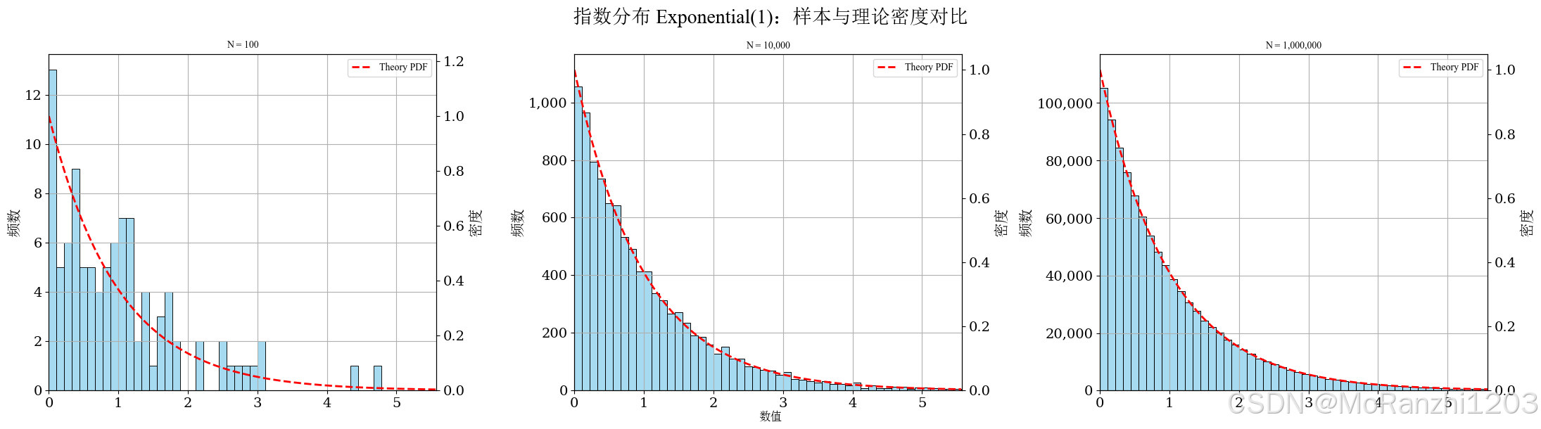
plot_continuous_samples(
title='指数分布 Exponential(1)',
sampler=lambda n: np.random.exponential(scale=1, size=n),
dist=expon(scale=1),
bins=50,
q_low=0.0,
q_high=0.995,
hard_clip=(0, 10)
)
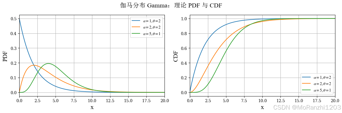
1.4 伽马分布 (Gamma)
Gamma 分布可以看作是指数分布的推广,在等待多个独立事件总耗时的建模中非常常见。它在贝叶斯统计、可靠性分析和正值随机变量建模中也有广泛应用。其密度函数为:
f(x∣α,θ)=1Γ(α)θαxα−1e−x/θ,x>0 f(x|\alpha,\theta) = \frac{1}{\Gamma(\alpha)\theta^\alpha} x^{\alpha-1} e^{-x/\theta}, \quad x>0 f(x∣α,θ)=Γ(α)θα1xα−1e−x/θ,x>0
这里 α\alphaα 是形状参数,θ\thetaθ 是尺度参数。特别地,当 α=1\alpha = 1α=1 时,Gamma 分布退化为指数分布。随着参数变化,Gamma 分布可以表现出不同程度的右偏,是理解参数如何影响分布形态的典型例子。
python
from scipy.stats import gamma
gamma_dists = [gamma(a=1, scale=2), gamma(a=2, scale=2), gamma(a=5, scale=1)]
gamma_labels = [r'$\alpha=1,\theta=2$', r'$\alpha=2,\theta=2$', r'$\alpha=5,\theta=1$']
plot_continuous_theory(
title='伽马分布 Gamma',
dist_list=gamma_dists,
labels=gamma_labels,
x_range=(0, 20)
)
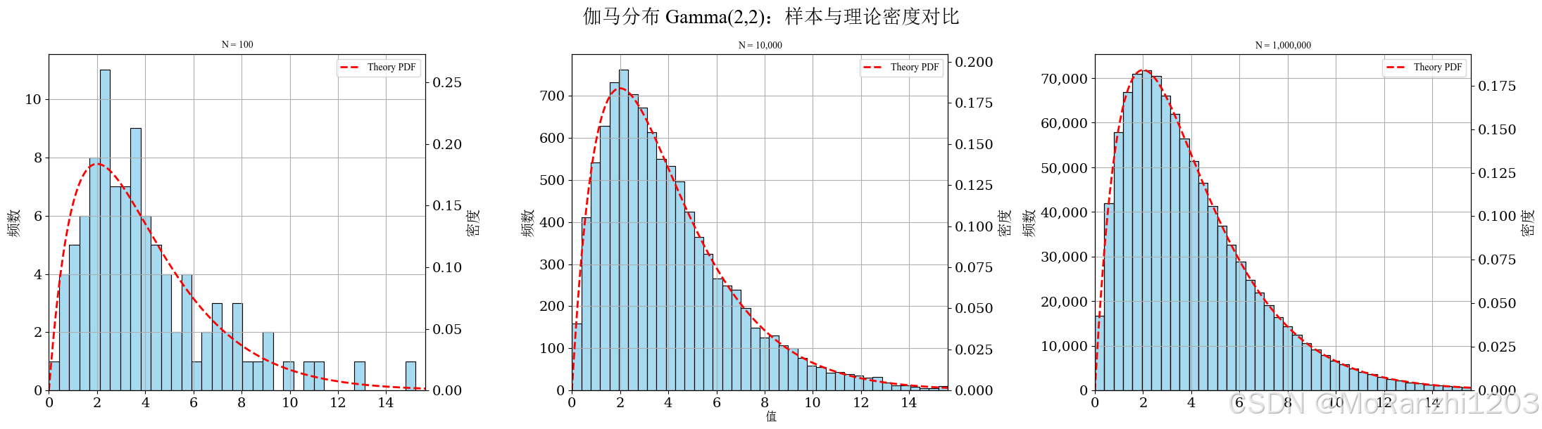
plot_continuous_samples(
title='伽马分布 Gamma(2,2)',
sampler=lambda n: np.random.gamma(shape=2, scale=2, size=n),
dist=gamma(a=2, scale=2),
bins=40,
q_low=0.0,
q_high=0.995,
hard_clip=(0, 20),
xlabel='值'
)
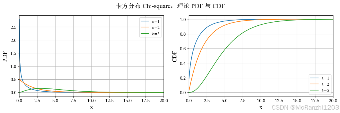
1.5 卡方分布 (Chi-square)
卡方分布在统计推断中十分常见,尤其是在假设检验、拟合优度检验和方差分析中。它定义在正半轴上,形状由自由度控制。它的密度函数是:
f(x∣k)=12k/2Γ(k/2)xk/2−1e−x/2,x>0 f(x|k) = \frac{1}{2^{k/2}\Gamma(k/2)} x^{k/2-1} e^{-x/2}, \quad x>0 f(x∣k)=2k/2Γ(k/2)1xk/2−1e−x/2,x>0
其中 kkk 表示自由度。自由度较小时,分布右偏明显;随着自由度增大,分布逐渐向右移动,曲线也会变得更平滑。由于卡方分布与正态变量平方和密切相关,因此它在很多统计量的分布推导中都会出现。
python
from scipy.stats import chi2
chi2_dists = [chi2(df=1), chi2(df=2), chi2(df=5)]
chi2_labels = [r'$k=1$', r'$k=2$', r'$k=5$']
plot_continuous_theory(
title='卡方分布 Chi-square',
dist_list=chi2_dists,
labels=chi2_labels,
x_range=(0, 20)
)
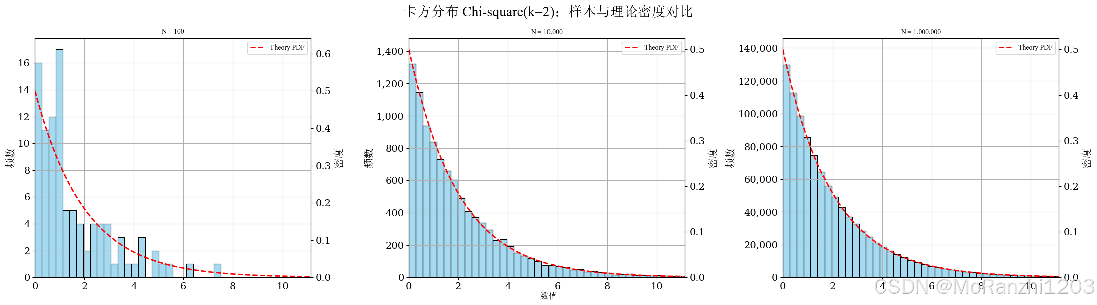
plot_continuous_samples(
title='卡方分布 Chi-square(k=2)',
sampler=lambda n: np.random.chisquare(df=2, size=n),
dist=chi2(df=2),
bins=40,
q_low=0.0,
q_high=0.995,
hard_clip=(0, 20)
)
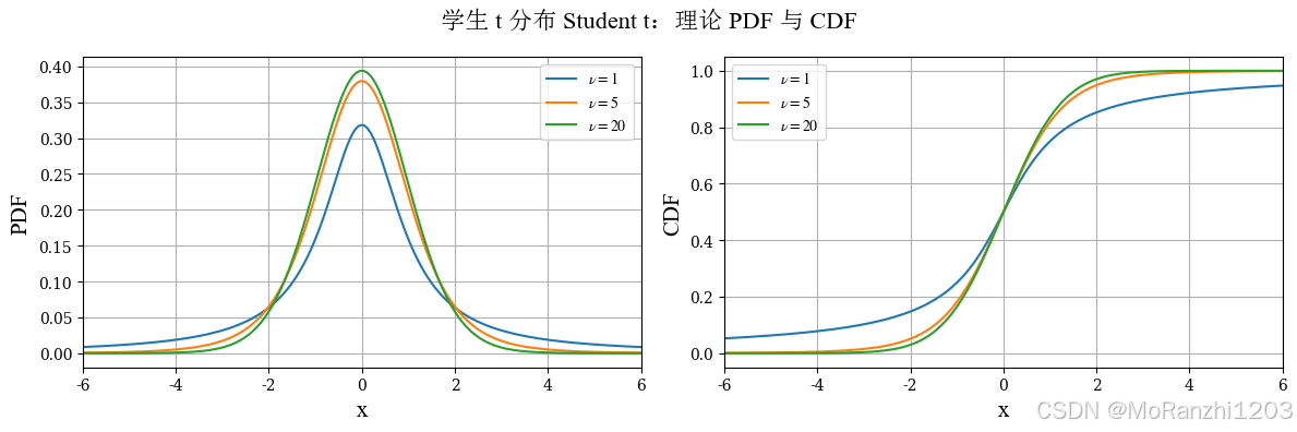
1.6 学生 t 分布 (Student t)
学生 t 分布常用于总体方差未知、样本量较小的情形。它与正态分布类似,都具有对称结构,但 t 分布的尾部更厚,因此能够更好地反映小样本条件下的不确定性。其密度函数为:
f(x∣ν)=Γ(ν+12)νπΓ(ν2)(1+x2ν)−(ν+1)/2 f(x|\nu) = \frac{\Gamma(\frac{\nu+1}{2})}{\sqrt{\nu\pi}\Gamma(\frac{\nu}{2})} \left(1+\frac{x^2}{\nu}\right)^{-(\nu+1)/2} f(x∣ν)=νπ Γ(2ν)Γ(2ν+1)(1+νx2)−(ν+1)/2
其中 ν\nuν 是自由度。自由度越小,尾部越厚;随着自由度增大,t 分布逐渐逼近标准正态分布。这也是为什么在样本量较大时,t 分布和正态分布的差异会减弱。
python
from scipy.stats import t
t_dists = [t(df=1), t(df=5), t(df=20)]
t_labels = [r'$\nu=1$', r'$\nu=5$', r'$\nu=20$']
plot_continuous_theory(
title='学生 t 分布 Student t',
dist_list=t_dists,
labels=t_labels,
x_range=(-6, 6)
)
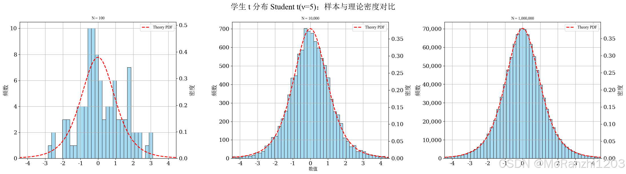
plot_continuous_samples(
title='学生 t 分布 Student t(ν=5)',
sampler=lambda n: np.random.standard_t(df=5, size=n),
dist=t(df=5),
bins=48,
q_low=0.005,
q_high=0.995,
hard_clip=(-6, 6)
)
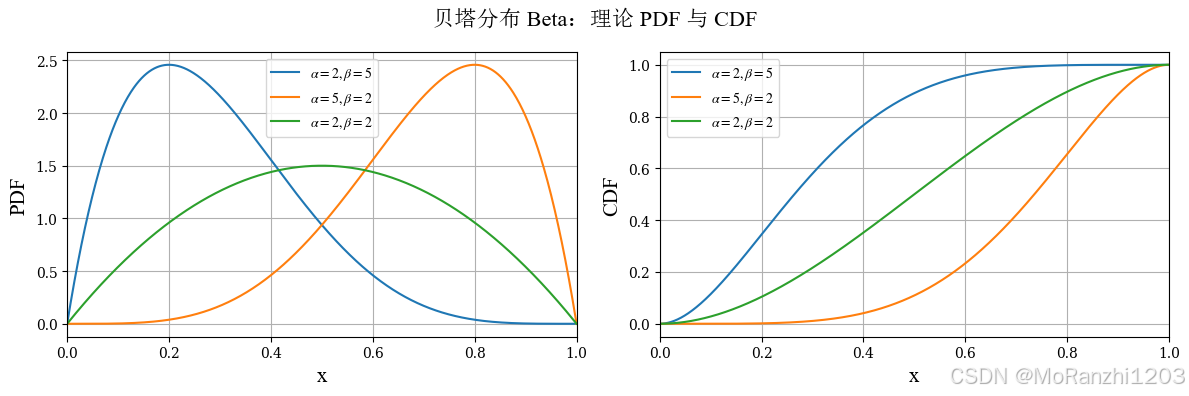
1.7 贝塔分布 (Beta)
贝塔分布定义在区间 (0,1)(0,1)(0,1) 上,因此非常适合用来描述概率、比例、转化率等变量。它在贝叶斯统计中常作为二项分布参数的先验分布。其密度函数为:
f(x∣α,β)=Γ(α+β)Γ(α)Γ(β)xα−1(1−x)β−1,0<x<1 f(x|\alpha,\beta) = \frac{\Gamma(\alpha+\beta)}{\Gamma(\alpha)\Gamma(\beta)} x^{\alpha-1} (1-x)^{\beta-1}, \quad 0<x<1 f(x∣α,β)=Γ(α)Γ(β)Γ(α+β)xα−1(1−x)β−1,0<x<1
贝塔分布的特点在于形状非常灵活。不同参数组合下,它可以表现为左偏、右偏、对称等多种形态。对于需要建模"取值介于 0 和 1 之间"的变量时,贝塔分布是一个常用选择。
python
from scipy.stats import beta
beta_dists = [beta(a=2, b=5), beta(a=5, b=2), beta(a=2, b=2)]
beta_labels = [r'$\alpha=2,\beta=5$', r'$\alpha=5,\beta=2$', r'$\alpha=2,\beta=2$']
plot_continuous_theory(
title='贝塔分布 Beta',
dist_list=beta_dists,
labels=beta_labels,
x_range=(0, 1)
)
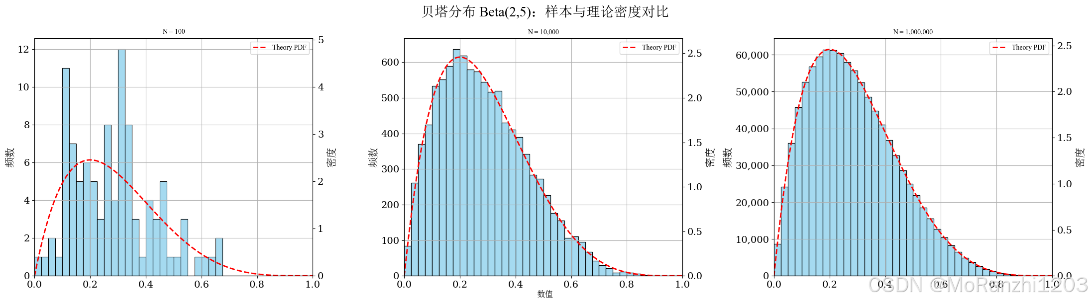
plot_continuous_samples(
title='贝塔分布 Beta(2,5)',
sampler=lambda n: np.random.beta(a=2, b=5, size=n),
dist=beta(a=2, b=5),
bins=40,
fixed_range=(0, 1)
)
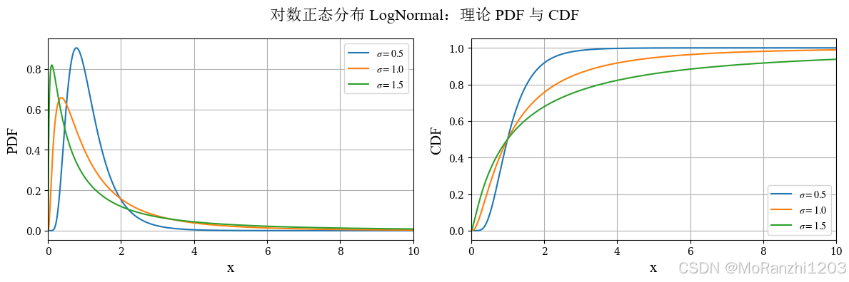
1.8 对数正态分布 (LogNormal)
如果一个随机变量的对数服从正态分布,那么这个随机变量本身就服从对数正态分布。它非常适合用来建模右偏、正值、具有乘法增长特征的数据,例如收入、价格、部分生物指标等。其密度函数为:
f(x∣μ,σ)=1xσ2πexp(−(lnx−μ)22σ2),x>0 f(x|\mu,\sigma) = \frac{1}{x\sigma\sqrt{2\pi}} \exp\Big(-\frac{(\ln x - \mu)^2}{2\sigma^2}\Big), \quad x>0 f(x∣μ,σ)=xσ2π 1exp(−2σ2(lnx−μ)2),x>0
python
from scipy.stats import lognorm

lognorm_dists = [
    lognorm(s=0.5, scale=np.exp(0)),
    lognorm(s=1.0, scale=np.exp(0)),
    lognorm(s=1.5, scale=np.exp(0))
]
lognorm_labels = [r'$\sigma=0.5$', r'$\sigma=1.0$', r'$\sigma=1.5$']

plot_continuous_theory(
    title='对数正态分布 LogNormal',
    dist_list=lognorm_dists,
    labels=lognorm_labels,
    x_range=(0, 10)
)
plot_continuous_samples(
    title='对数正态分布 LogNormal(0,1)',
    sampler=lambda n: np.random.lognormal(mean=0, sigma=1, size=n),
    dist=lognorm(s=1, scale=np.exp(0)),
    bins=40,
    q_low=0.001,
    q_high=0.99,
    hard_clip=(0, 12)
)
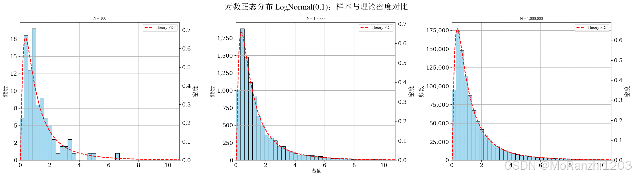
与正态分布相比,对数正态分布明显右偏,且尾部较长。样本图中通常可以观察到少量较大的取值,这也是该分布的一个典型特征。
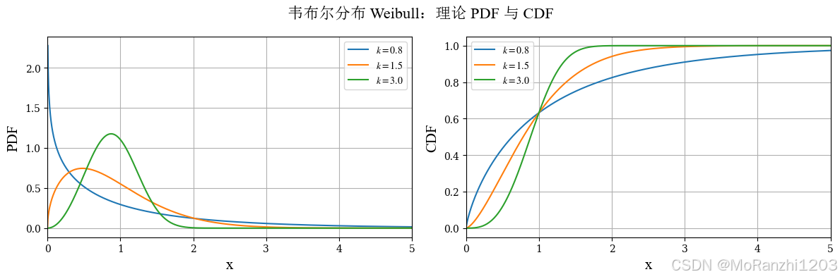
1.9 韦布尔分布 (Weibull)
也称韦伯分布。它在寿命分析和可靠性工程中应用广泛,能够灵活描述不同失效模式下的数据分布。其密度函数可以写为:
f(x∣k)=kxk−1e−xk,x>0 f(x|k) = k x^{k-1} e^{-x^k}, \quad x>0 f(x∣k)=kxk−1e−xk,x>0
韦布尔分布的形状参数 kkk 会显著影响分布的形态,因此它比指数分布具有更高的灵活性。它常用于建模设备寿命、故障时间等正值随机变量。
python
from scipy.stats import weibull_min
weibull_dists = [weibull_min(c=0.8), weibull_min(c=1.5), weibull_min(c=3.0)]
weibull_labels = [r'$k=0.8$', r'$k=1.5$', r'$k=3.0$']
plot_continuous_theory(
title='韦布尔分布 Weibull',
dist_list=weibull_dists,
labels=weibull_labels,
x_range=(0, 5)
)
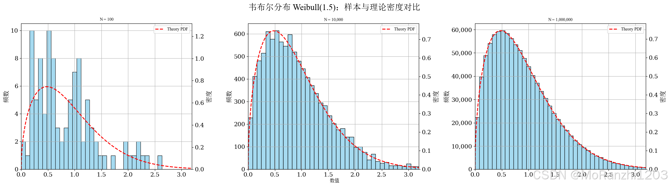
plot_continuous_samples(
title='韦布尔分布 Weibull(1.5)',
sampler=lambda n: np.random.weibull(a=1.5, size=n),
dist=weibull_min(c=1.5),
bins=40,
q_low=0.0,
q_high=0.995,
hard_clip=(0, 5)
)
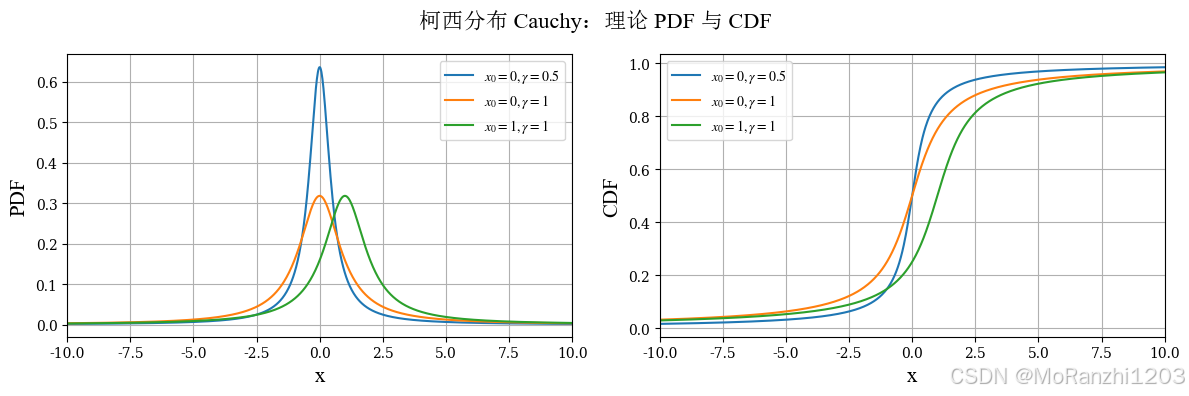
1.10 柯西分布 (Cauchy)
柯西分布是一个很有代表性的重尾分布。它的曲线看起来与正态分布有些相似,但本质上差别很大。柯西分布没有期望,也没有方差,这使它在统计学中经常被用来作为"异常重尾行为"的典型例子。其密度函数为:
f(x∣x0,γ)=1πγ1+(x−x0γ)2 f(x|x_0,\gamma) = \frac{1}{\pi\gamma1+(\\frac{x-x_0}{\\gamma})\^2} f(x∣x0,γ)=πγ1+(γx−x0)21
python
from scipy.stats import cauchy

cauchy_dists = [cauchy(loc=0, scale=0.5), cauchy(loc=0, scale=1), cauchy(loc=1, scale=1)]
cauchy_labels = [r'$x_0=0,\gamma=0.5$', r'$x_0=0,\gamma=1$', r'$x_0=1,\gamma=1$']

plot_continuous_theory(
    title='柯西分布 Cauchy',
    dist_list=cauchy_dists,
    labels=cauchy_labels,
    x_range=(-10, 10)
)
plot_continuous_samples(
    title='柯西分布 Cauchy(0,1)',
    sampler=lambda n: np.random.standard_cauchy(size=n),
    dist=cauchy(),
    bins=40,
    q_low=0.05,
    q_high=0.95,
    hard_clip=(-8, 8)
)
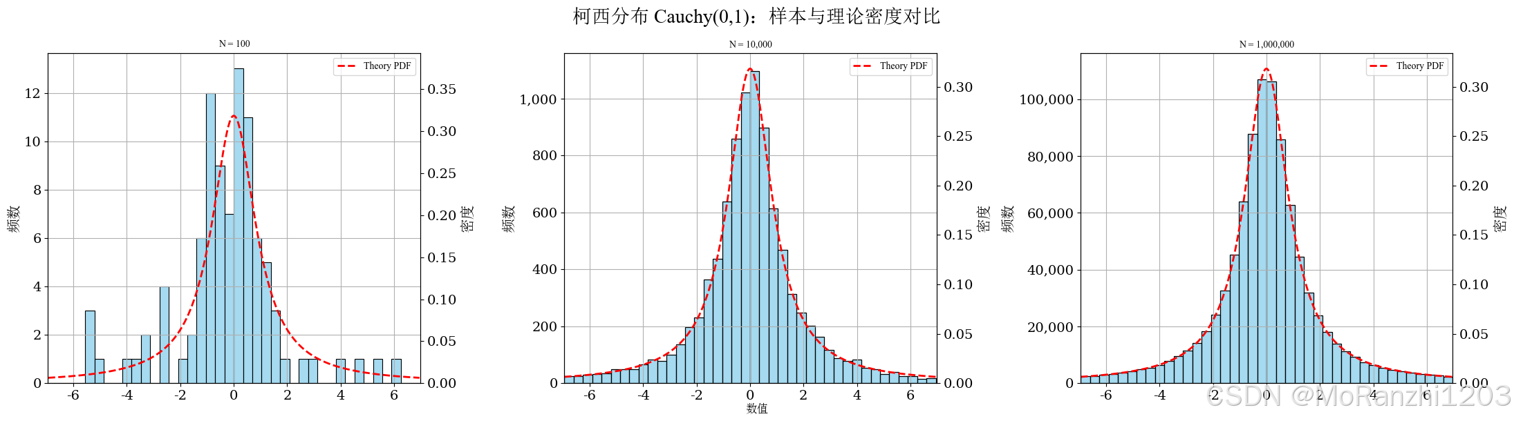
由于尾部极重,样本中容易出现极端值。为了使主体区域更清晰,绘图时通常需要对横轴范围进行较强的分位数裁剪,否则少量极端值会显著拉伸坐标范围,导致主体部分几乎看不清。
1.11 拉普拉斯分布 (Laplace)
拉普拉斯分布也称双指数分布。与正态分布相比,它的中心更尖,尾部也更厚,因此在某些鲁棒建模和稀疏建模问题中很有意义。其密度函数为:
f(x∣μ,b)=12bexp(−∣x−μ∣b) f(x|\mu,b) = \frac{1}{2b} \exp\Big(-\frac{|x-\mu|}{b}\Big) f(x∣μ,b)=2b1exp(−b∣x−μ∣)
python
from scipy.stats import laplace

laplace_dists = [laplace(loc=0, scale=0.5), laplace(loc=0, scale=1), laplace(loc=1, scale=1)]
laplace_labels = [r'$\mu=0,b=0.5$', r'$\mu=0,b=1$', r'$\mu=1,b=1$']
plot_continuous_theory(
    title='拉普拉斯分布 Laplace',
    dist_list=laplace_dists,
    labels=laplace_labels,
    x_range=(-6, 6)
)
plot_continuous_samples(
    title='拉普拉斯分布 Laplace(0,1)',
    sampler=lambda n: np.random.laplace(loc=0, scale=1, size=n),
    dist=laplace(loc=0, scale=1),
    bins=40,
    q_low=0.005,
    q_high=0.995,
    hard_clip=(-6, 6)
)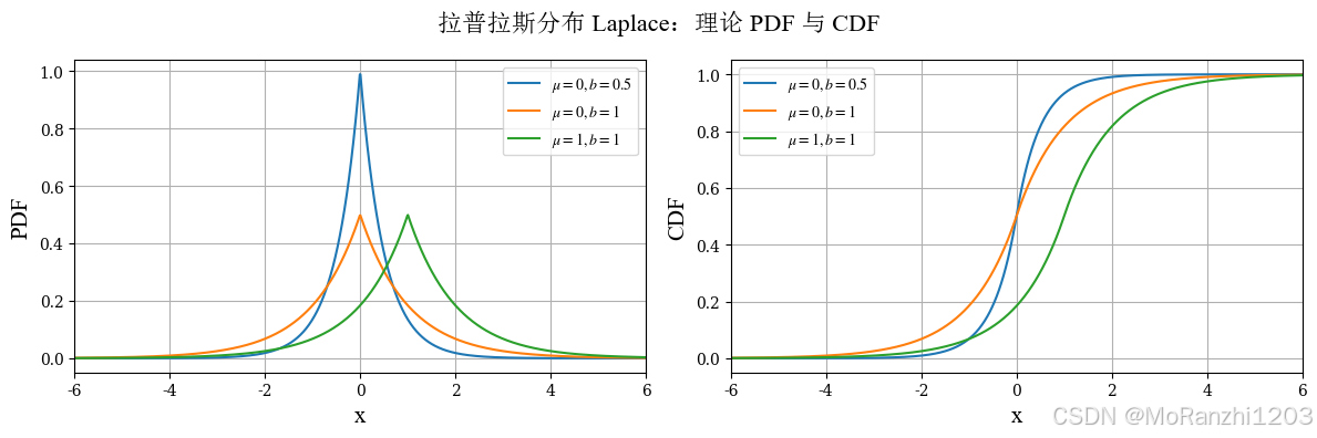
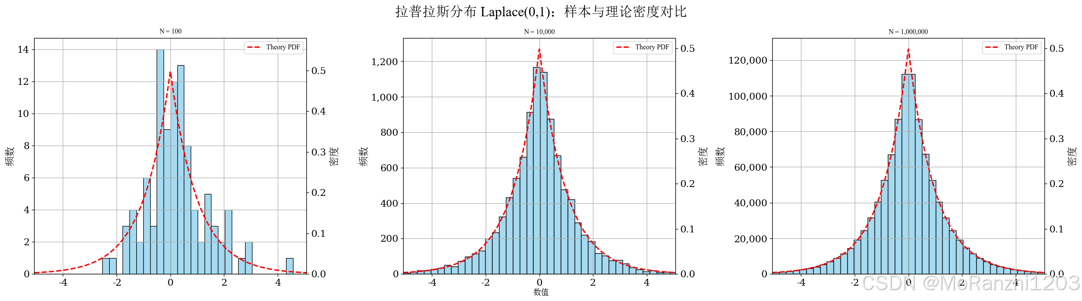
从图像上看,拉普拉斯分布的峰值更集中,说明数据更容易聚集在中心附近;同时尾部衰减速度又慢于正态分布,因此极端值出现的概率相对更高。
1.12 瑞利分布 (Rayleigh)
瑞利分布定义在正半轴上,常用于信号处理、无线通信以及二维高斯向量模长的建模。其密度函数为:
f(x∣σ)=xσ2exp(−x2/(2σ2)),x>0 f(x|\sigma) = \frac{x}{\sigma^2} \exp(-x^2/(2\sigma^2)), \quad x>0 f(x∣σ)=σ2xexp(−x2/(2σ2)),x>0
python
from scipy.stats import rayleigh

rayleigh_dists = [rayleigh(scale=0.5), rayleigh(scale=1), rayleigh(scale=2)]
rayleigh_labels = [r'$\sigma=0.5$', r'$\sigma=1$', r'$\sigma=2$']
plot_continuous_theory(
    title='瑞利分布 Rayleigh',
    dist_list=rayleigh_dists,
    labels=rayleigh_labels,
    x_range=(0, 8)
)
plot_continuous_samples(
    title='瑞利分布 Rayleigh(1)',
    sampler=lambda n: np.random.rayleigh(scale=1, size=n),
    dist=rayleigh(scale=1),
    bins=40,
    q_low=0.0,
    q_high=0.995,
    hard_clip=(0, 5)
)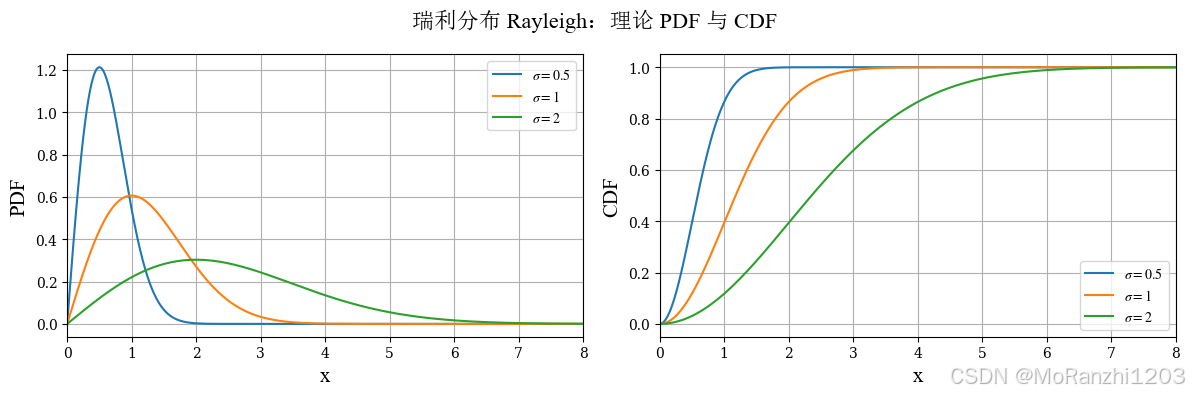
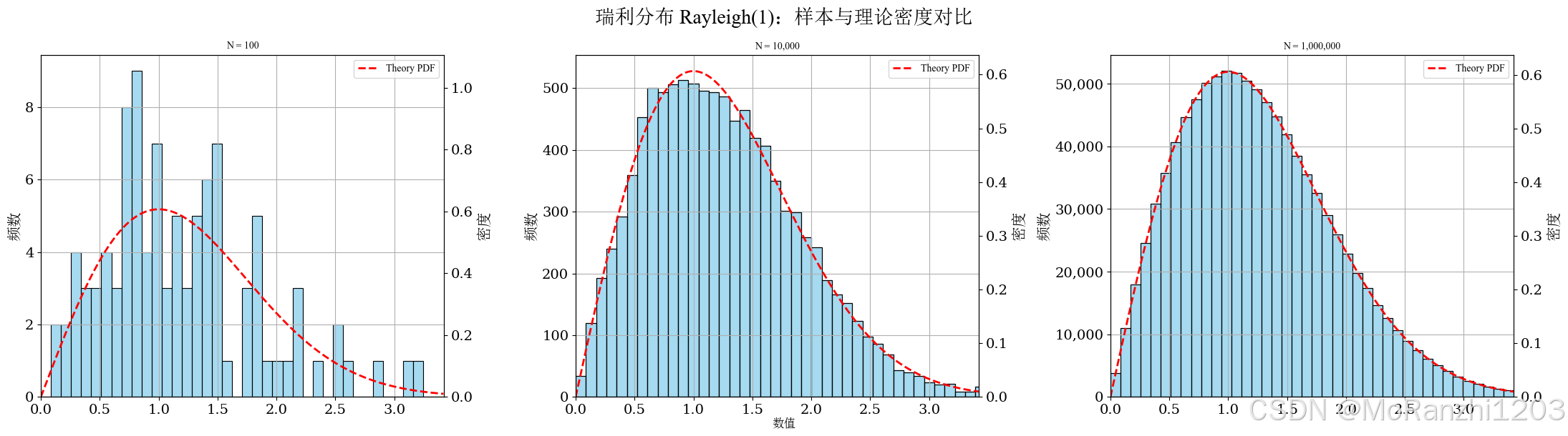
它的图像通常呈现单峰右偏特征,适合描述非负幅值类变量。与指数分布、Gamma 分布等正值分布相比,瑞利分布具有自己的峰值位置和衰减方式。
1.13 三角分布 (Triangular)
三角分布适用于只知道最小值、最大值和最可能值,但缺少更完整统计信息的场景。它常见于工程估算、项目管理和简化模拟中。其密度函数为:
f(x∣a,b,c)={2(x−a)(b−a)(c−a),a≤x<c2(b−x)(b−a)(b−c),c≤x≤b f(x|a,b,c) = \begin{cases} \frac{2(x-a)}{(b-a)(c-a)}, & a \le x < c\\ \frac{2(b-x)}{(b-a)(b-c)}, & c \le x \le b \end{cases} f(x∣a,b,c)={(b−a)(c−a)2(x−a),(b−a)(b−c)2(b−x),a≤x<cc≤x≤b
python
from scipy.stats import triang

triang_dists = [
    triang(c=0.2, loc=0, scale=10),
    triang(c=0.5, loc=0, scale=10),
    triang(c=0.8, loc=0, scale=10)
]
triang_labels = [r'$mode=2$', r'$mode=5$', r'$mode=8$']

plot_continuous_theory(
    title='三角分布 Triangular',
    dist_list=triang_dists,
    labels=triang_labels,
    x_range=(0, 10)
)
plot_continuous_samples(
    title='三角分布 Triangular(0,5,10)',
    sampler=lambda n: np.random.triangular(left=0, mode=5, right=10, size=n),
    dist=triang(c=0.5, loc=0, scale=10),
    bins=40,
    fixed_range=(0, 10)
)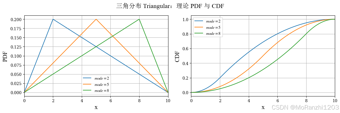
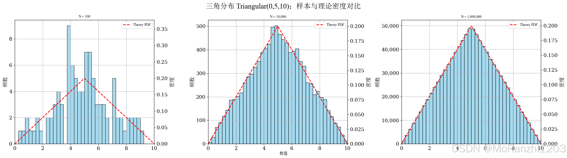
三角分布的图像由线性上升和线性下降两部分构成,峰值位置对应最可能值。由于它只依赖少量参数,因此在数据不足但需要快速建模时非常实用。
2. 离散型概率分布
离散型分布用于描述取值为有限个或可数个离散点的随机变量,通常通过概率质量函数(PMF)和累积分布函数(CDF)表示。相比连续型分布,离散型分布更适合描述次数、个数和试验结果等问题。
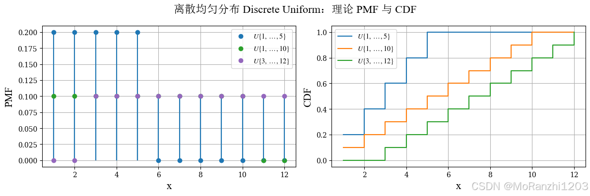
2.1 离散均匀分布 (Discrete Uniform)
离散均匀分布表示在一组有限整数中,每个取值的概率完全相同。它可以看作连续均匀分布在离散情形下的对应形式。它的概率质量函数为:
P(X=x)=1n,x=1,2,...,n P(X=x) = \frac{1}{n}, \quad x = 1,2,...,n P(X=x)=n1,x=1,2,...,n
它常用于简单的随机取整问题,例如掷骰子、整数抽样等,也是离散型概率质量函数最直观的例子之一。
python
from scipy.stats import randint
du_dists = [randint(1, 6), randint(1, 11), randint(3, 13)]
du_labels = [r'$U\{1,\dots,5\}$', r'$U\{1,\dots,10\}$', r'$U\{3,\dots,12\}$']
plot_discrete_theory(
title='离散均匀分布 Discrete Uniform',
dist_list=du_dists,
labels=du_labels,
x_values=np.arange(1, 13)
)
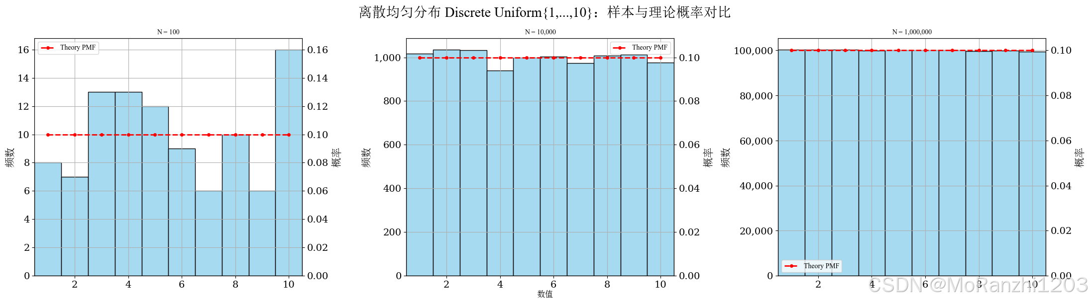
plot_discrete_samples(
title='离散均匀分布 Discrete Uniform{1,...,10}',
sampler=lambda n: np.random.randint(1, 11, size=n),
dist=randint(1, 11),
x_values=np.arange(1, 11)
)
2.2 二项分布 (Binomial)
二项分布描述进行 nnn 次独立伯努利试验后成功次数的分布,是离散型分布中最基础的一类。其概率质量函数为:
P(X=k)=(nk)pk(1−p)n−k,k=0,1,...,n P(X=k)=\binom{n}{k}p^k(1-p)^{n-k}, \quad k=0,1,...,n P(X=k)=(kn)pk(1−p)n−k,k=0,1,...,n
参数 nnn 表示试验次数,ppp 表示单次成功概率。当 p=0.5p=0.5p=0.5 时,分布较为对称;当 ppp 偏离 0.5 时,分布会表现出偏斜。二项分布广泛用于建模重复试验中的成功次数问题。
python
from scipy.stats import binom
binom_dists = [binom(n=10, p=0.3), binom(n=10, p=0.5), binom(n=10, p=0.7)]
binom_labels = [r'$n=10,p=0.3$', r'$n=10,p=0.5$', r'$n=10,p=0.7$']
plot_discrete_theory(
title='二项分布 Binomial',
dist_list=binom_dists,
labels=binom_labels,
x_values=np.arange(0, 11)
)
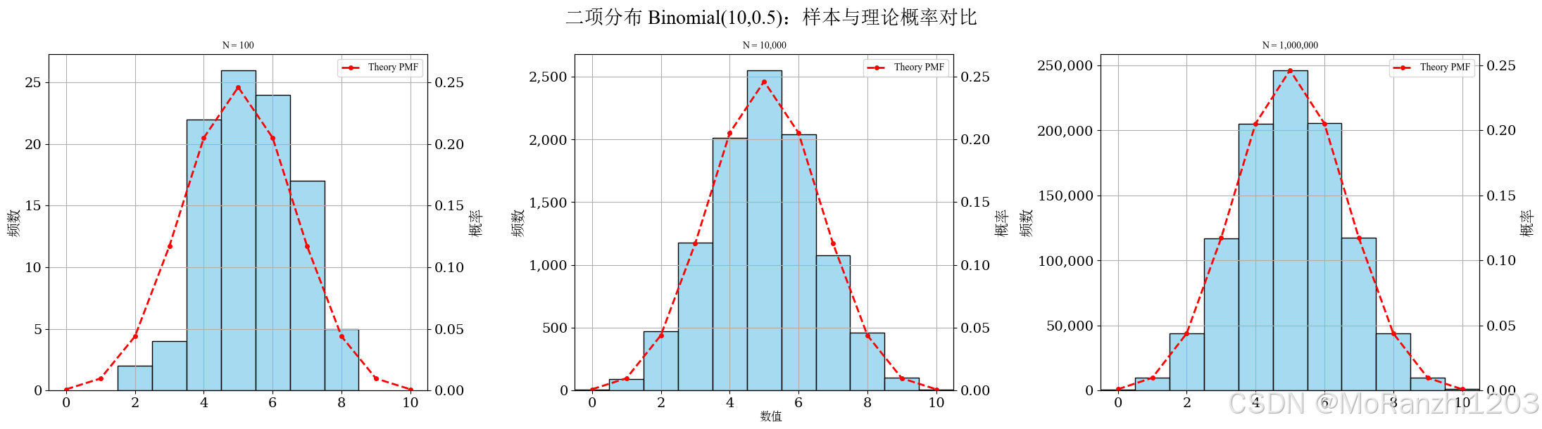
plot_discrete_samples(
title='二项分布 Binomial(10,0.5)',
sampler=lambda n: np.random.binomial(10, 0.5, size=n),
dist=binom(n=10, p=0.5),
x_values=np.arange(0, 11)
)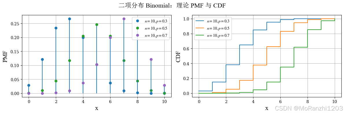
当 p=0.5p = 0.5p=0.5 时,分布通常更接近对称;当 ppp 偏离 0.5 时,分布会表现出更明显的偏斜。
2.3 泊松分布 (Poisson)
泊松分布用于描述单位时间、单位区域或单位空间内某事件发生次数的分布,适合处理计数问题。其概率质量函数为:
P(X=k)=λke−λk!,k=0,1,2,... P(X=k)=\frac{\lambda^k e^{-\lambda}}{k!}, \quad k=0,1,2,... P(X=k)=k!λke−λ,k=0,1,2,...
参数 λ\lambdaλ 控制平均发生次数。λ\lambdaλ 越大,分布峰值越向右移动,整体形态也更平滑。泊松分布与指数分布关系密切,前者描述事件次数,后者描述事件间隔时间。
python
from scipy.stats import poisson
poisson_dists = [poisson(mu=2), poisson(mu=4), poisson(mu=8)]
poisson_labels = [r'$\lambda=2$', r'$\lambda=4$', r'$\lambda=8$']
plot_discrete_theory(
title='泊松分布 Poisson',
dist_list=poisson_dists,
labels=poisson_labels,
x_values=np.arange(0, 21)
)
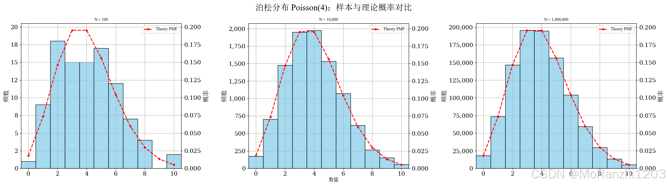
plot_discrete_samples(
title='泊松分布 Poisson(4)',
sampler=lambda n: np.random.poisson(4, size=n),
dist=poisson(mu=4),
cdf_threshold=0.995,
start=0
)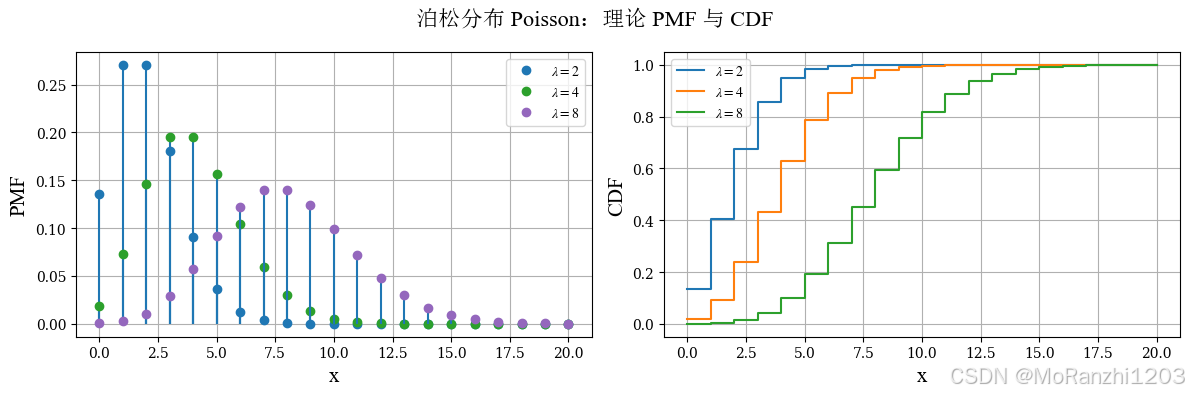
泊松分布与指数分布之间还有非常紧密的联系:泊松分布关注的是事件"发生了多少次",而指数分布则关注"下一次事件还要等多久"。
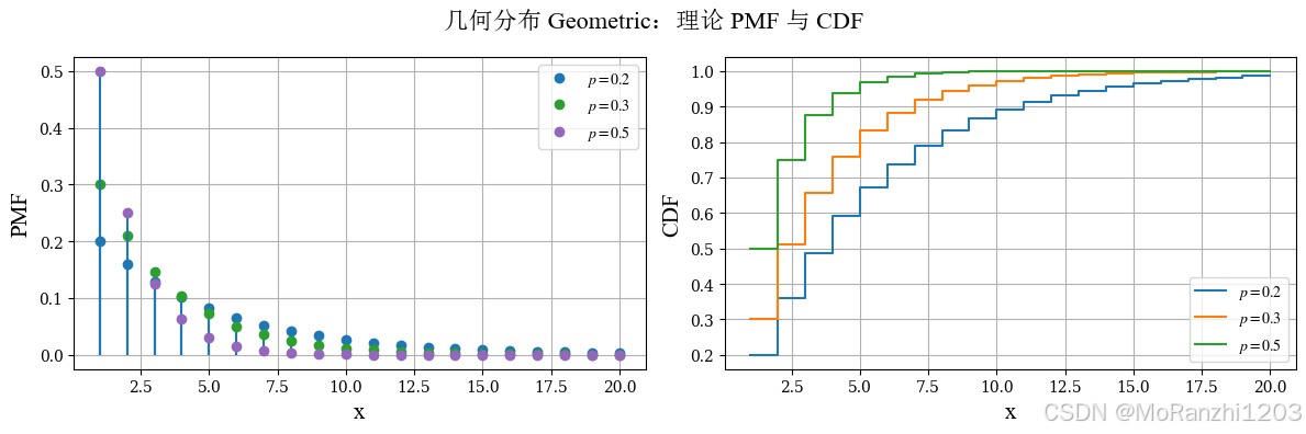
2.4 几何分布 (Geometric)
几何分布描述的是在独立重复试验中,第一次成功出现在第几次试验。它适合建模"重复尝试直到首次成功"的过程。它的概率质量函数为:
P(X=k)=p(1−p)k−1,k=1,2,3,... P(X=k)=p(1-p)^{k-1}, \quad k=1,2,3,... P(X=k)=p(1−p)k−1,k=1,2,3,...
几何分布是离散型等待时间分布的典型代表,并且同样具有无记忆性。它与指数分布之间存在明显的对应关系:一个用于离散时间,一个用于连续时间。
python
from scipy.stats import geom
geom_dists = [geom(p=0.2), geom(p=0.3), geom(p=0.5)]
geom_labels = [r'$p=0.2$', r'$p=0.3$', r'$p=0.5$']
plot_discrete_theory(
title='几何分布 Geometric',
dist_list=geom_dists,
labels=geom_labels,
x_values=np.arange(1, 21)
)
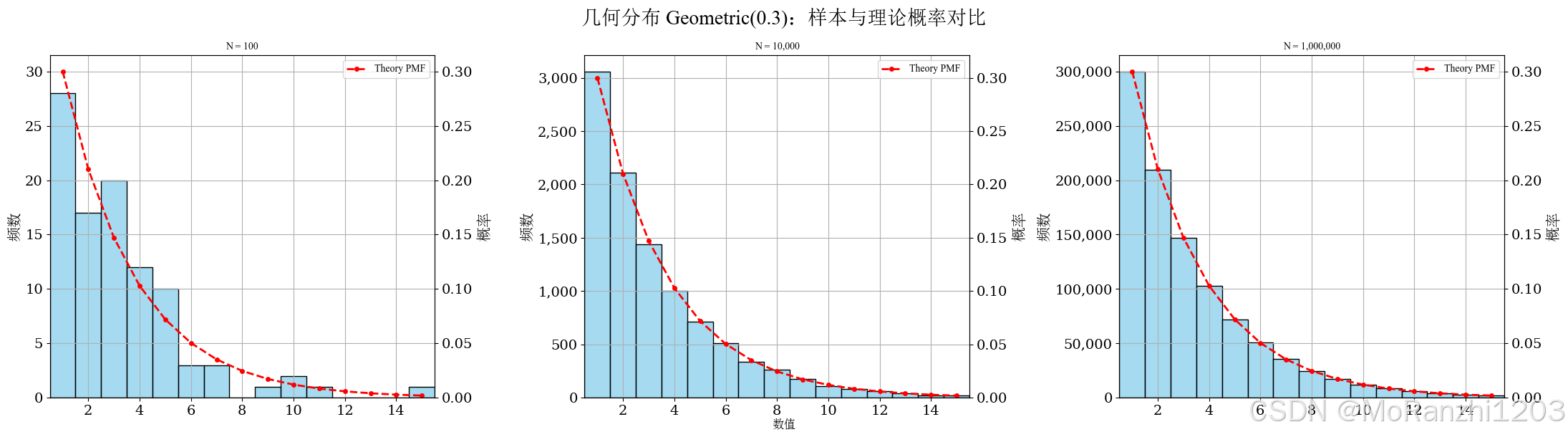
plot_discrete_samples(
title='几何分布 Geometric(0.3)',
sampler=lambda n: np.random.geometric(0.3, size=n),
dist=geom(p=0.3),
cdf_threshold=0.995,
start=1
)
2.5 负二项分布 (Negative Binomial)
负二项分布可以理解为几何分布的推广,用于描述为了获得固定次数的成功,需要经历多少次失败,或者等价地,需要多少次试验。
P(X=k)=(k+r−1k)pr(1−p)k,k=0,1,2,... P(X=k)=\binom{k+r-1}{k}p^r(1-p)^k, \quad k=0,1,2,... P(X=k)=(kk+r−1)pr(1−p)k,k=0,1,2,...
python
from scipy.stats import nbinom
nbinom_dists = [nbinom(n=3, p=0.3), nbinom(n=5, p=0.3), nbinom(n=5, p=0.5)]
nbinom_labels = [r'$r=3,p=0.3$', r'$r=5,p=0.3$', r'$r=5,p=0.5$']
plot_discrete_theory(
title='负二项分布 Negative Binomial',
dist_list=nbinom_dists,
labels=nbinom_labels,
x_values=np.arange(0, 31)
)
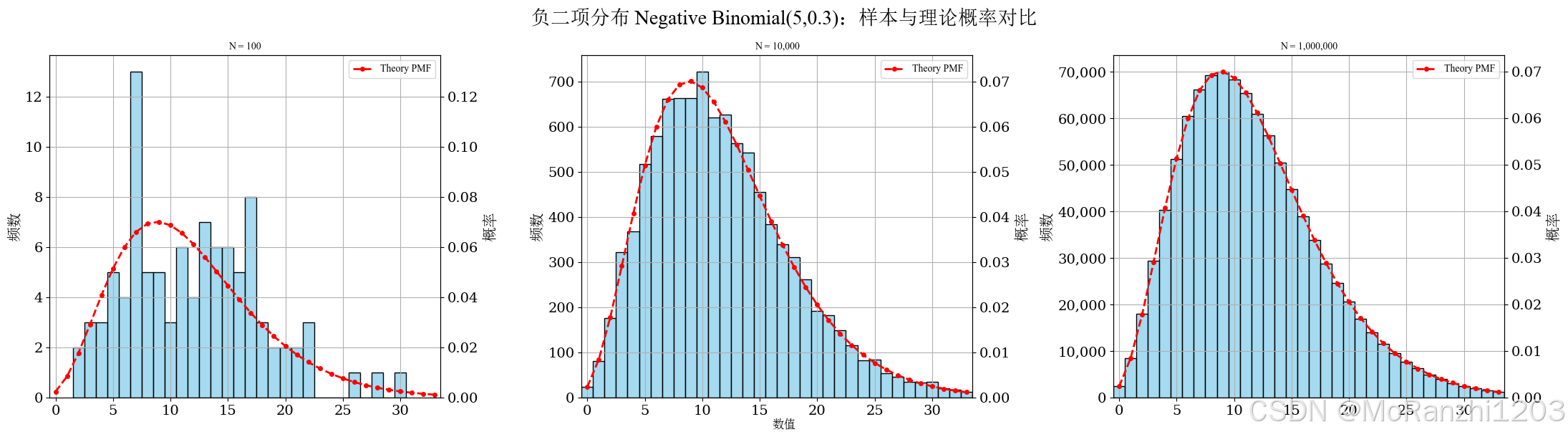
plot_discrete_samples(
title='负二项分布 Negative Binomial(5,0.3)',
sampler=lambda n: np.random.negative_binomial(5, 0.3, size=n),
dist=nbinom(n=5, p=0.3),
cdf_threshold=0.995,
start=0
)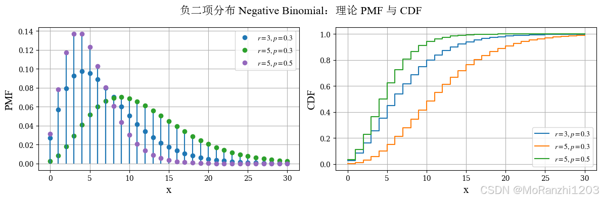
相比几何分布,负二项分布能够描述更复杂的重复试验过程,因此在建模中更具灵活性。参数变化会显著影响分布的偏斜程度和尾部长度。
3. 总结
本文基于统一的绘图函数,对常见连续型与离散型概率分布进行了可视化整理。相比单独记忆公式,这种方式更有助于理解分布的形状、参数作用以及样本与理论之间的关系。
从理论图像到样本对照图,可以清楚看到不同分布在形态上的差异,也可以观察到样本量增大时经验分布对理论分布的逼近过程。这种从公式到图像、从理论到样本的对应关系,是理解概率分布时非常重要的一环。
如果后续需要扩展更多分布,只需在当前框架上补充分布对象和采样函数即可,整体结构可以保持不变。这也是统一封装绘图函数的一个直接优势。