目录
[4.1 load_data_dblp-数据处理](#4.1 load_data_dblp-数据处理)
[5.1 adj_to_bias](#5.1 adj_to_bias)
第一点:矩阵乘法实现路径累积(图论中经典的"图的幂"概念在GNN中的应用)
图神经网络概览:图神经网络分享系列-概览
上一篇文章:图神经网络分享系列-HAN(Heterogeneous Graph Attention Network)(一)
本章内容主要进行实战
github链接:https://github.com/Jhy1993/HAN
一、概览
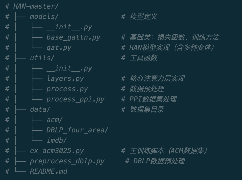
1、整体架构
2、数据集说明(本篇以acm为例)
ACM数据集包含3025篇论文,分为3类:
-
类别0: Neural Network (神经网络)
-
类别1: Data Mining (数据挖掘)
-
类别2: Computer Vision (计算机视觉)
元路径 (Meta-paths):
-
PAP: Paper-Author-Paper (通过作者相连的论文)
-
PLP: Paper-Label-Paper (通过标签相连的论文)
二、主函数
1、超参数
batch_size = 1 # 批次大小(由于是全图训练,设为1)
nb_epochs = 200 # 最大训练轮数
patience = 100 # 早停耐心值(验证集性能不提升的最大轮数)
lr = 0.005 # 学习率
l2_coef = 0.001 # L2正则化系数(防止过拟合)
hid_units = 8 #隐藏层单元数列表,隐藏单元数为8
n_heads = 8, 1 #第一层: 8个注意力头; 输出层: 1个注意力头
2、激活函数
elu
3、模型
HeteGAT_multi
4、加载数据集
4.1 load_data_dblp-数据处理
python
# 加载ACM数据集
adj_list, fea_list, y_train, y_val, y_test, train_mask, val_mask, test_mask = load_data_dblp()
print('adj_list:{},fea_list:{},y_train:{}, y_val:{}, y_test:{}, train_mask:{}, val_mask:{}, test_mask:{}'.format(
    adj_list[0].shape,fea_list[0].shape,y_train.shape, y_val.shape, y_test.shape,
        train_mask.shape, val_mask.shape, test_mask.shape))

adj_list:(3025, 3025),fea_list:(3025, 1870),y_train:(3025, 3), y_val:(3025, 3), y_test:(3025, 3), train_mask:(3025,), val_mask:(3025,), test_mask:(3025,)
python
def sample_mask(idx, l):
    """
    创建训练/验证/测试掩码

    用于标识哪些节点有标签,哪些节点无标签。
    半监督学习中只有有标签的节点参与损失计算。

    参数:
        idx: 有标签节点的索引(数组或列表)
        l: 节点总数

    返回:
        mask: 布尔掩码数组,shape [l]
              mask[i] = True 表示节点i有标签
    """
    mask = np.zeros(l)
    mask[idx] = 1
    return np.array(mask, dtype=np.bool_)

def load_data_dblp(path='data/acm/ACM3025.mat'):
    """
    加载ACM数据集

    从.mat文件中读取:
    - 节点特征 (feature)
    - 节点标签 (label)
    - 元路径邻接矩阵 (PAP, PLP)
    - 训练/验证/测试集划分索引

    参数:
        path: .mat文件路径

    返回:
        rownetworks: 元路径邻接矩阵列表 [PAP, PLP]
        truefeatures_list: 节点特征列表(复制3份)
        y_train/val/test: 训练/验证/测试标签
        train/val/test_mask: 对应的掩码
    """
    # 读取.mat文件
    data = sio.loadmat(path)

    # 这是一份处理好的数据,有这些列
    #dict_keys(['__header__', '__version__', '__globals__', 'PTP', 'PLP', 'PAP','feature', 'label', 'train_idx', 'val_idx', 'test_idx'])

    # 获取标签和特征
    # truelabels: [3025, 3] - 每行是一个one-hot编码的标签(3类)
    # truefeatures: [3025, 1870] - 3025个节点,每个节点1870维特征
    truelabels, truefeatures = data['label'], data['feature'].astype(float)

    # 节点数量
    N = truefeatures.shape[0]

    # =================================================================
    # 构建元路径邻接矩阵
    # =================================================================
    # PAP: Paper-Author-Paper (通过共同作者相连的论文)
    # PLP: Paper-Label-Paper (通过共同标签相连的论文)
    # 减去np.eye(N)是为了去除自环
    rownetworks = [
        data['PAP'] - np.eye(N),  # PAP元路径邻接矩阵
        data['PLP'] - np.eye(N)   # PLP元路径邻接矩阵
    ]

    # =================================================================
    # 获取标签和划分
    # =================================================================
    y = truelabels  # 标签 [3025, 3]

    # 训练/验证/测试集索引
    train_idx = data['train_idx']   # 训练集索引
    val_idx = data['val_idx']       # 验证集索引
    test_idx = data['test_idx']     # 测试集索引

    # 创建掩码
    train_mask = sample_mask(train_idx, y.shape[0])
    val_mask = sample_mask(val_idx, y.shape[0])
    test_mask = sample_mask(test_idx, y.shape[0])

    # =================================================================
    # 构建标签矩阵(与掩码配合使用)
    # =================================================================
    # 初始化为全0,有标签的位置填充真实标签
    y_train = np.zeros(y.shape)
    y_val = np.zeros(y.shape)
    y_test = np.zeros(y.shape)

    # 填充有标签节点的值
    y_train[train_mask, :] = y[train_mask, :]
    y_val[val_mask, :] = y[val_mask, :]
    y_test[test_mask, :] = y[test_mask, :]

    # 打印数据集信息
    print('y_train:{}, y_val:{}, y_test:{}, train_idx:{}, val_idx:{}, test_idx:{}'.format(
        y_train.shape, y_val.shape, y_test.shape,
        train_idx.shape, val_idx.shape, test_idx.shape))

    # 特征列表(复制3份,对应3个元路径的输入)
    # 注:实际只用了fea_list的前2个元素
    truefeatures_list = [truefeatures, truefeatures, truefeatures]

    return rownetworks, truefeatures_list, y_train, y_val, y_test, train_mask, val_mask, test_mask
5、数据预处理
python
# =================================================================================
# 数据预处理
# =================================================================================
# 获取基本信息
nb_nodes = fea_list[0].shape[0]  # 节点数量 (3025)
ft_size = fea_list[0].shape[1]  # 特征维度 (1870)
nb_classes = y_train.shape[1]    # 类别数量 (3)

# =================================================================
# 维度扩展
# =================================================================
# TensorFlow期望的输入维度: [batch_size, nb_nodes, feature_dim]
# 需要在第0维添加batch维度
fea_list = [fea[np.newaxis] for fea in fea_list]      # shape: [1, 3025, 1870]
adj_list = [adj[np.newaxis] for adj in adj_list]      # shape: [1, 3025, 3025]
y_train = y_train[np.newaxis]                          # shape: [1, 3025, 3]
y_val = y_val[np.newaxis]                             # shape: [1, 3025, 3]
y_test = y_test[np.newaxis]                           # shape: [1, 3025, 3]
train_mask = train_mask[np.newaxis]                   # shape: [1, 3025]
val_mask = val_mask[np.newaxis]                       # shape: [1, 3025]
test_mask = test_mask[np.newaxis]                     # shape: [1, 3025]

# =================================================================
# 构建邻接矩阵偏置
# =================================================================
# 将邻接矩阵转换为偏置矩阵,用于注意力机制
# 非邻居位置设为-1e9,邻居位置设为0
# 这样在Softmax后,非邻居的注意力权重几乎为0
biases_list = [process.adj_to_bias(adj, [nb_nodes], nhood=1) for adj in adj_list]
5.1 adj_to_bias
python
def adj_to_bias(adj, sizes, nhood=1):
    """
    将邻接矩阵转换为偏置矩阵,用于图神经网络的注意力机制。

    该函数首先扩展邻接矩阵以计算n-hop邻居可达性,然后将其转换为
    二值化偏置向量。在注意力机制中,不可达的节点对将被赋予极大的
    负值,从而使其注意力权重接近于零。

    Args:
        adj: 邻接矩阵,形状为 [graph_num, nodes, nodes]。
        sizes: 列表,每个元素表示对应图中节点的数量。
        nhood: 邻居跳数,默认为1。表示计算可达性时考虑的图的邻居阶数。

    Returns:
        偏置矩阵,形状与输入邻接矩阵相同。对于不可达的节点对(i,j),
        返回值为-1e9;对于可达的节点对,返回值为0。
    """
    print(adj.shape)
    # adj.shape: (1, 3025, 3025)
    # sizes = (1, 3025)

    nb_graphs = adj.shape[0]  # 获取图的数量
    mt = np.empty(adj.shape)  # 初始化矩阵存储可达性信息
    for g in range(nb_graphs):
        print("graph:", g)
        mt[g] = np.eye(adj.shape[1])  # 初始化为单位矩阵,表示0-hop可达性
        print(mt[g].shape)
        for _ in range(nhood):
            # 计算n-hop邻居可达性:矩阵乘法实现路径累积
            mt[g] = np.matmul(mt[g], (adj[g] + np.eye(adj.shape[1])))
            print(mt[g].shape,adj.shape,g,adj[g].shape,np.eye(adj.shape[1]).shape)
        print(sizes[g])
        # 二值化:可达的节点对设为1,否则保持0
        for i in range(sizes[g]):
            for j in range(sizes[g]):
                if mt[g][i][j] > 0.0:
                    mt[g][i][j] = 1.0
    # 返回偏置矩阵:可达节点对为0,不可达节点对为-1e9
    return -1e9 * (1.0 - mt)
这个代码有3个点说一下
**第一点:**矩阵乘法实现路径累积(图论中经典的"图的幂"概念在GNN中的应用)
- 通过矩阵乘法实现路径累积:(A @ B)ij = Σk Aik * Bkj
- 矩阵A、B,做乘法,当A和B是二值矩阵(0或1)时:
- 如果存在节点k使得
A[i][k] = 1且B[k][j] = 1 - 则
(A @ B)[i][j] ≥ 1,表示存在从i通过k到j的路径
- 如果存在节点k使得
- 所以如果
(A @ B)[i][j] = 2,则说明从i到j有2条路径可达。 为了方便理解,举个例子假设一个3节点矩阵,从0-1有1条边,1-2有1条边adj = \[0, 1, 0,0, 0, 1,
0, 0, 0\]
- 初始状态 (0-hop): 自身链接,各有1条边,每个节点只能到达自己
- 矩阵A、B,做乘法,当A和B是二值矩阵(0或1)时:
mt = I = \[1, 0, 0,
0, 1, 0,
0, 0, 1\]
-
-
- 第1次乘法 (1-hop):
-
mt = mt @ (adj + I) = \[1, 0, 0, \[1, 1, 0,
0, 1, 0, @ 0, 1, 1,
0, 0, 1\]\] \[0, 0, 1\]
= \[1, 1, 0,
0, 1, 1,
0, 0, 1\]
- 节点0可到达0和1
- 节点1可到达1和2
- 节点2可到达2
-
-
- 第2次乘法 (2-hop):
-
mt = mt @ (adj + I)
= \[1, 2, 1,
0, 1, 2,
0, 0, 1\]
- 节点0可通过1条边到达节点2(路径:0→1->2)
- 数值2表示有2条路径(比如节点0到节点1: 0→1和0->1->1)
**第二点:**为什么需要nhood次循环
每次矩阵乘法相当于:
- 第1次: 计算直接邻居(1-hop可达)
- 第2次: 计算邻居的邻居(2-hop可达)
- 第n次: 计算n-hop内可达的节点
循环nhood次后,mt[g][i][j] > 0 表示节点i可以在nhood跳内到达节点j。
**第三点:**最后的二值化
将累积的路径数量简化为二值:可达=1,不可达=0,不关心具体有多少条路径。
6、TensorFlow计算图构建
-
输入占位符定义
-
前向传播
-
损失函数计算
python
# 创建默认计算图
with tf1.Graph().as_default():
    # 创建输入命名空间
    with tf1.name_scope('input'):
        # =================================================================
        # 定义输入占位符
        # =================================================================
        # 特征输入列表(对应多个元路径)
        # shape: [batch_size, nb_nodes, ft_size]
        ftr_in_list = [tf1.placeholder(dtype=tf1.float32,
                                      shape=(batch_size, nb_nodes, ft_size),
                                      name='ftr_in_{}'.format(i))
                       for i in range(len(fea_list))]

        # 邻接矩阵偏置输入列表
        # shape: [batch_size, nb_nodes, nb_nodes]
        bias_in_list = [tf1.placeholder(dtype=tf1.float32,
                                       shape=(batch_size, nb_nodes, nb_nodes),
                                       name='bias_in_{}'.format(i))
                        for i in range(len(biases_list))]

        # 标签输入 (one-hot编码)
        # shape: [batch_size, nb_nodes, nb_classes]
        lbl_in = tf1.placeholder(dtype=tf1.int32, shape=(
            batch_size, nb_nodes, nb_classes), name='lbl_in')

        # 掩码输入(标识哪些节点有标签)
        # shape: [batch_size, nb_nodes]
        msk_in = tf1.placeholder(dtype=tf1.int32, shape=(batch_size, nb_nodes),
                                name='msk_in')

        # Dropout占位符
        attn_drop = tf1.placeholder(dtype=tf1.float32, shape=(), name='attn_drop')  # 注意力dropout
        ffd_drop = tf1.placeholder(dtype=tf1.float32, shape=(), name='ffd_drop')    # 前馈dropout

        # 训练/推理模式标志
        is_train = tf1.placeholder(dtype=tf1.bool, shape=(), name='is_train')

    # =================================================================
    # 前向传播
    # =================================================================
    # 调用模型inference函数
    # 返回: logits(分类结果), final_embedding(节点嵌入), att_val(元路径注意力权重)
    logits, final_embedding, att_val = model.inference(
        ftr_in_list, nb_classes, nb_nodes, is_train,
        attn_drop, ffd_drop,
        bias_mat_list=bias_in_list,
        hid_units=hid_units, n_heads=n_heads,
        residual=residual, activation=nonlinearity)

    # =================================================================
    # 计算损失函数
    # =================================================================
    # 重塑logits和标签以便计算损失
    log_resh = tf1.reshape(logits, [-1, nb_classes])      # [batch*nodes, classes]
    lab_resh = tf1.reshape(lbl_in, [-1, nb_classes])      # [batch*nodes, classes]
    msk_resh = tf1.reshape(msk_in, [-1])                  # [batch*nodes]

    # 计算带掩码的softmax交叉熵损失(只计算有标签节点)
    loss = model.masked_softmax_cross_entropy(log_resh, lab_resh, msk_resh)

    # 计算带掩码的准确率
    accuracy = model.masked_accuracy(log_resh, lab_resh, msk_resh)

    # =================================================================
    # 定义训练操作
    # =================================================================
    train_op = model.training(loss, lr, l2_coef)

    # 创建模型保存/加载器
    saver = tf1.train.Saver()

    # 初始化所有变量
    init_op = tf1.group(tf1.global_variables_initializer(),
                       tf1.local_variables_initializer())

    # =================================================================
    # 早停变量
    # =================================================================
    vlss_mn = np.inf       # 最佳验证损失(越小越好)
    vacc_mx = 0.0          # 最佳验证准确率(越大越好)
    curr_step = 0          # 当前连续未改善的轮数
7、训练阶段
python
# =================================================================================
# 训练模型
# =================================================================================
# 启动TensorFlow会话
with tf1.Session(config=config) as sess:
    # 初始化变量
    sess.run(init_op)

    # 训练和验证损失/准确率的累积变量
    train_loss_avg = 0
    train_acc_avg = 0
    val_loss_avg = 0
    val_acc_avg = 0

    # =================================================================
    # 训练循环
    # =================================================================
    for epoch in range(nb_epochs):
        # -----------------------------------------------------------------
        # 训练阶段
        # -----------------------------------------------------------------
        tr_step = 0
        tr_size = fea_list[0].shape[0]  # 样本数量

        # 由于batch_size=1,每个epoch只训练一次(整个图)
        while tr_step * batch_size < tr_size:
            # 准备训练数据
            # 特征
            fd1 = {i: d[tr_step * batch_size:(tr_step + 1) * batch_size]
                   for i, d in zip(ftr_in_list, fea_list)}
            # 邻接矩阵偏置
            fd2 = {i: d[tr_step * batch_size:(tr_step + 1) * batch_size]
                   for i, d in zip(bias_in_list, biases_list)}
            # 标签、掩码、训练标志
            fd3 = {lbl_in: y_train[tr_step * batch_size:(tr_step + 1) * batch_size],
                   msk_in: train_mask[tr_step * batch_size:(tr_step + 1) * batch_size],
                   is_train: True,
                   attn_drop: 0.6,   # 训练时使用dropout
                   ffd_drop: 0.6}

            # 合并字典
            fd = fd1
            fd.update(fd2)
            fd.update(fd3)

            # 执行训练
            _, loss_value_tr, acc_tr, att_val_train = sess.run(
                [train_op, loss, accuracy, att_val],
                feed_dict=fd)

            # 累积损失和准确率
            train_loss_avg += loss_value_tr
            train_acc_avg += acc_tr
            tr_step += 1

        # -----------------------------------------------------------------
        # 验证阶段
        # -----------------------------------------------------------------
        vl_step = 0
        vl_size = fea_list[0].shape[0]

        while vl_step * batch_size < vl_size:
            # 准备验证数据
            fd1 = {i: d[vl_step * batch_size:(vl_step + 1) * batch_size]
                   for i, d in zip(ftr_in_list, fea_list)}
            fd2 = {i: d[vl_step * batch_size:(vl_step + 1) * batch_size]
                   for i, d in zip(bias_in_list, biases_list)}
            fd3 = {lbl_in: y_val[vl_step * batch_size:(vl_step + 1) * batch_size],
                   msk_in: val_mask[vl_step * batch_size:(vl_step + 1) * batch_size],
                   is_train: False,
                   attn_drop: 0.0,   # 验证时不使用dropout
                   ffd_drop: 0.0}

            fd = fd1
            fd.update(fd2)
            fd.update(fd3)

            # 执行验证
            loss_value_vl, acc_vl = sess.run([loss, accuracy],
                                             feed_dict=fd)
            val_loss_avg += loss_value_vl
            val_acc_avg += acc_vl
            vl_step += 1

        # 打印训练/验证结果
        print('Epoch: {}, att_val: {}'.format(epoch, np.mean(att_val_train, axis=0)))
        print('Training: loss = %.5f, acc = %.5f | Val: loss = %.5f, acc = %.5f' %
              (train_loss_avg / tr_step, train_acc_avg / tr_step,
               val_loss_avg / vl_step, val_acc_avg / vl_step))

        # -----------------------------------------------------------------
        # 早停检查
        # -----------------------------------------------------------------
        # 如果验证准确率提升或验证损失下降
        if val_acc_avg / vl_step >= vacc_mx or val_loss_avg / vl_step <= vlss_mn:
            # 如果同时满足准确率提升和损失下降,保存最佳模型
            if val_acc_avg / vl_step >= vacc_mx and val_loss_avg / vl_step <= vlss_mn:
                vacc_early_model = val_acc_avg / vl_step
                vlss_early_model = val_loss_avg / vl_step
                saver.save(sess, checkpt_file)

            # 更新最佳记录
            vacc_mx = np.max((val_acc_avg / vl_step, vacc_mx))
            vlss_mn = np.min((val_loss_avg / vl_step, vlss_mn))
            curr_step = 0
        else:
            # 连续未改善轮数+1
            curr_step += 1
            # 如果达到早停耐心值,停止训练
            if curr_step == patience:
                print('Early stop! Min loss: ', vlss_mn,
                      ', Max accuracy: ', vacc_mx)
                print('Early stop model validation loss: ',
                      vlss_early_model, ', accuracy: ', vacc_early_model)
                break

        # 重置累积变量
        train_loss_avg = 0
        train_acc_avg = 0
        val_loss_avg = 0
        val_acc_avg = 0
鉴于内容过多,下一篇会详细介绍模型部分~