CVPR 2026 | C²FG：用分数差异分析提高条件生成中CFG的引导

作者： vivo BlueImage Lab
摘要： 针对扩散生成中长期使用的固定 CFG scale 机制存在不合理论的假设，该工作从 score 差异随扩散时间衰减的角度首次提出了 时间自适应的指数控制函数（C²FG）。这一 training-free、plug-and-play 引导策略在 DiT、SiT、Stable Diffusion 等多种框架上均稳定带来显著 FID 降低与 IS 提升，并可与 interval guidance/auto guidance 等方法正交叠加。实验证明，在 ImageNet 条件生成任务中，C²FG 在多个架构与采样器配置下达到了行业领先的生成质量。对应的论文已被 CVPR 接收！

该工作由vivo BlueImage Lab，上海交通大学共同完成。

本文入选 CVPR 2026

CVPR（IEEE/CVF Conference on Computer Vision and Pattern Recognition）IEEE国际计算机视觉与模式识别会议，主要内容是计算机视觉与模式识别技术。

论文主页：arxiv.org/abs/2603.08...

一、为什么固定 CFG scale 不够好？

标准 CFG： <math xmlns="http://www.w3.org/1998/Math/MathML"> ϵ ^ ω ( x t , t , y ) = ϵ ^ ∅ ( x t , t ) + ω ( ϵ ^ c ( x t , t , y ) − ϵ ^ ∅ ( x t , t ) ) . \hat\epsilon_\omega(x_t,t,y)=\hat\epsilon_{\emptyset}(x_t,t)+\omega\big(\hat\epsilon_{c}(x_t,t,y)-\hat\epsilon_{\emptyset}(x_t,t)\big). </math>ϵ^ω(xt,t,y)=ϵ^∅(xt,t)+ω(ϵ^c(xt,t,y)−ϵ^∅(xt,t)). 常见做法使用固定 <math xmlns="http://www.w3.org/1998/Math/MathML"> ω \omega </math>ω，但它默认"条件/无条件差异在所有时间步同等重要"。我们的理论与实证显示：这种差异在扩散时间上是动态变化的 ，因此固定 <math xmlns="http://www.w3.org/1998/Math/MathML"> ω \omega </math>ω 难以同时兼顾早期结构形成与后期精确对齐。

二、核心理论（VP-SDE 重点）：score discrepancy 的严格上界（论文 Theorem 1）

VP-SDE 前向扩散： <math xmlns="http://www.w3.org/1998/Math/MathML"> d x t = − 1 2 β ( t ) x t d t + β ( t ) d w t . dx_t=-\frac{1}{2}\beta(t)x_tdt+\sqrt{\beta(t)}dw_t. </math>dxt=−21β(t)xtdt+β(t) dwt.

Theorem 1（VP-SDE Score MSE Bound）

假设样本空间有界且闭。令 <math xmlns="http://www.w3.org/1998/Math/MathML"> p ( x , t ) p(x,t) </math>p(x,t) 与 <math xmlns="http://www.w3.org/1998/Math/MathML"> p ~ ( x , t ) \tilde p(x,t) </math>p~(x,t) 为由初始分布 <math xmlns="http://www.w3.org/1998/Math/MathML"> p ( x 0 ) p(x_0) </math>p(x0) 与 <math xmlns="http://www.w3.org/1998/Math/MathML"> p ~ ( x 0 ) \tilde p(x_0) </math>p~(x0) 诱导的时刻 <math xmlns="http://www.w3.org/1998/Math/MathML"> t t </math>t 的密度（论文中取 <math xmlns="http://www.w3.org/1998/Math/MathML"> p ~ ( x , t ) = p ( x , t ∣ y ) \tilde p(x,t)=p(x,t\mid y) </math>p~(x,t)=p(x,t∣y)）。则 score 差异满足一致上界： <math xmlns="http://www.w3.org/1998/Math/MathML"> ∣ ∇ log ⁡ p ( x , t ) − ∇ log ⁡ p ~ ( x , t ) ∣ ≤ α ( t ) σ 2 ( t ) C , ∀ x ∈ s u p p , t ≥ 0 , |\nabla\log p(x,t)-\nabla\log \tilde p(x,t)| \le \frac{\alpha(t)}{\sigma^2(t)}C,\quad \forall x\in \mathrm{supp},\ t\ge 0, </math>∣∇logp(x,t)−∇logp~(x,t)∣≤σ2(t)α(t)C,∀x∈supp, t≥0, 其中 <math xmlns="http://www.w3.org/1998/Math/MathML"> C C </math>C 为常数， <math xmlns="http://www.w3.org/1998/Math/MathML"> α ( t ) = exp ⁡ ( − 1 2 ∫ 0 t β s d s ) , σ ( t ) = α ( t ) ∫ 0 t β s α 2 ( s ) d s . \alpha(t)=\exp\Big(-\frac{1}{2}\int_0^t\beta_sds\Big),\quad \sigma(t)=\alpha(t)\sqrt{\int_0^t\frac{\beta_s}{\alpha^2(s)}ds}. </math>α(t)=exp(−21∫0tβsds),σ(t)=α(t)∫0tα2(s)βsds . 重参数化 <math xmlns="http://www.w3.org/1998/Math/MathML"> t ′ = 1 2 ∫ 0 t β s d s t'=\frac{1}{2}\int_0^t\beta_sds </math>t′=21∫0tβsds 后（论文式(9)）： <math xmlns="http://www.w3.org/1998/Math/MathML"> ∣ ∇ log ⁡ p ( x , t ) − ∇ log ⁡ p ( x , t ∣ y ) ∣ ≤ e − t 1 − e − 2 t C , |\nabla\log p(x,t)-\nabla\log p(x,t\mid y)| \le \frac{e^{-t}}{1-e^{-2t}}C, </math>∣∇logp(x,t)−∇logp(x,t∣y)∣≤1−e−2te−tC, 当 <math xmlns="http://www.w3.org/1998/Math/MathML"> t t </math>t 较大时呈现 <math xmlns="http://www.w3.org/1998/Math/MathML"> O ( e − t ) O(e^{-t}) </math>O(e−t) 的指数衰减趋势。

结论： 在前向扩散中，条件/无条件分布会逐步"趋同"，其 score 差异上界随时间衰减；对应到反向采样，越接近数据（ <math xmlns="http://www.w3.org/1998/Math/MathML"> t → 0 t\to 0 </math>t→0）越需要更强、更精细的条件引导。

三、方法：C²FG（指数控制的 time-dependent CFG）

我们将固定 <math xmlns="http://www.w3.org/1998/Math/MathML"> ω \omega </math>ω 替换为时间控制函数： <math xmlns="http://www.w3.org/1998/Math/MathML"> ω ( t ) = ω 0 exp ⁡ ( λ ( 1 − t t max ⁡ ) ) . \omega(t)=\omega_0\exp\Big(\lambda\Big(1-\frac{t}{t_{\max}}\Big)\Big). </math>ω(t)=ω0exp(λ(1−tmaxt)). 并在采样时使用：
<math xmlns="http://www.w3.org/1998/Math/MathML" display="block"> ϵ ^ c ω ( x t ) = ϵ ^ ∅ ( x t ) + ω ( t ) [ ϵ ^ c ( x t ) − ϵ ^ ∅ ( x t ) ] . \hat{\boldsymbol{\epsilon}}_{\boldsymbol{c}}^\omega\left(\boldsymbol{x}t\right)=\hat{\boldsymbol{\epsilon}}{\varnothing}\left(\boldsymbol{x}t\right)+\omega(t)\left[\hat{\boldsymbol{\epsilon}}{\boldsymbol{c}}\left(\boldsymbol{x}t\right)-\hat{\boldsymbol{\epsilon}}{\varnothing}\left(\boldsymbol{x}_t\right)\right] . </math>ϵ^cω(xt)=ϵ^∅(xt)+ω(t)[ϵ^c(xt)−ϵ^∅(xt)].

为什么这种形式好用？

• 与理论与观测一致： 差异呈指数趋势，调度函数自然对齐；
• 连续可导更稳定： 比分段/线性更平滑；
• 只需两个超参： <math xmlns="http://www.w3.org/1998/Math/MathML"> ω 0 \omega_0 </math>ω0（最大强度）与 <math xmlns="http://www.w3.org/1998/Math/MathML"> λ \lambda </math>λ（衰减速率）；
• training-free、plug-and-play： 无需额外训练或外部分类器。

四、实验结果展示

Figure 1：理论预测的"时间趋势"在真实模型中成立

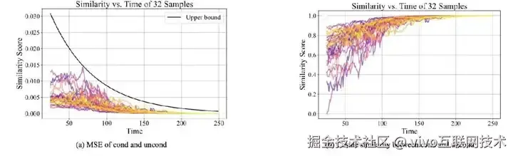
• (a) 条件与无条件 score 的 MSE 随时间变化，并被一个随 <math xmlns="http://www.w3.org/1998/Math/MathML"> t → + ∞ t\to+\infty </math>t→+∞ 逼近 0 的函数上界约束；
• (b) 余弦相似度在反向采样过程中下降，说明二者在幅值与方向上都逐渐分离。

Figure 2：CFG vs.C²FG 的采样流程比较

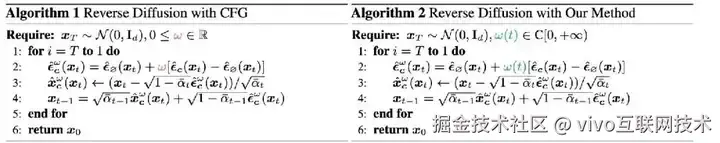
• CFG： <math xmlns="http://www.w3.org/1998/Math/MathML"> ω \omega </math>ω 为常数；
• C <math xmlns="http://www.w3.org/1998/Math/MathML"> 2 ^2 </math>2FG： <math xmlns="http://www.w3.org/1998/Math/MathML"> ω ( t ) \omega(t) </math>ω(t) 为随时间变化的衰减控制函数。

Figure 3：C²FG的直观示意（并解释 interval guidance 可视为特例/可融合）

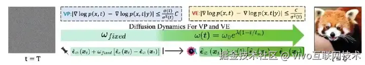
论文指出：区间 guidance 的"只在有效区间用引导"可以在我们的框架下得到解释；同时C²FG+ interval可以进一步减少不必要的模型评估开销（把引导放在更"有效"的阶段）。

Figure 4：2D Toy Example（更少 outliers，更贴近目标条件分布）

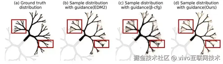
• (b) EDM2（ <math xmlns="http://www.w3.org/1998/Math/MathML"> ω = 1 \omega=1 </math>ω=1）出现 outliers；
• (c） <math xmlns="http://www.w3.org/1998/Math/MathML"> β \beta </math>β-CFG（ <math xmlns="http://www.w3.org/1998/Math/MathML"> α = β = 2 , ω = 1 \alpha=\beta=2,\ \omega=1 </math>α=β=2, ω=1）outliers 更多；
• (d) C <math xmlns="http://www.w3.org/1998/Math/MathML"> 2 ^2 </math>2FG（ <math xmlns="http://www.w3.org/1998/Math/MathML"> ω 0 = 1 , λ = 0.6 \omega_0=1,\ \lambda=0.6 </math>ω0=1, λ=0.6）outliers 更少，匹配目标更好。

Figure 5：ImageNet 质化对比（纹理更清晰、畸变更少）

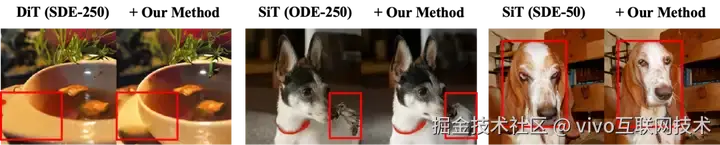
红框示例显示C²FG 能有效缓解失真与纹理模糊；在不同采样器与步数下都能保持一致改进。

ImageNet Class-Conditional（多架构、多分辨率、多采样器综合评估）

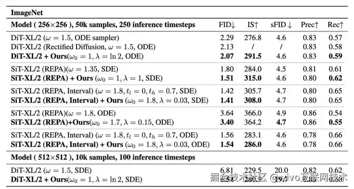
DiT-XL/2 (256×256, ODE)

• baseline：FID 2.29，IS 276.8
• C²FG（ω0=1, λ=ln2）：FID 2.07，IS 291.5

SiT-XL/2 (REPA, 256×256, SDE)（强基线也能继续提升）

• baseline：FID 1.80，IS 284.0
• C²FG（ω0=1, λ=1）：FID 1.51，IS 315.0

SiT-XL/2 (REPA, 256×256, SDE)（强基线也能继续提升）

• interval baseline：FID 1.42，IS 305.7
• interval +C²FG：FID 1.41，IS 308.0

DiT-XL/2 (512×512, SDE, 100 steps)

• baseline：FID 6.81，IS 229.5
• C²FG：FID 6.54，IS 280.9

引用：

C²FG：Control Classifier-Free Guidance via Score Discrepancy Analysis, CVPR 2026.

vivo BlueImage Lab
蓝图影像创新实验室 ，主要负责移动影像算法创新，包括图像/视频处理、图像/视频交互、图像/视频增强、多模态理解大模型等方面的技术前沿探索。

致力于不断提升vivo移动影像的算法能力，使用户能够拍摄出更加清晰、美观的照片和视频。同时积极探索增强现实、具身智能等新兴技术领域的应用，努力为用户提供更加丰富和便捷的影像体验。

欢迎持续关注 vivo 影像技术，获取前沿技术创新经验分享与热招岗位信息。