这是一个非常完整的LISA时空跃迁分析代码实现。让我从多个维度深度解析这个代码的技术内涵、应用场景和实现细节。
一、代码功能
1.1 代码目标
实现一个空间统计学 分析方法,通过局部莫兰指数(Local Moran's I) 分析中国省级行政区在多个时间点上的空间关联模式演变,并识别空间格局的动态变化规律。
1.2 主要模块
- 数据生成:模拟3个时间点的省级空间数据
- 空间权重构建:基于距离构建空间邻接矩阵
- LISA分析:计算局部空间自相关模式
- 时空跃迁分析:识别空间格局的动态变化
- 可视化呈现:空间分布地图+统计图表
二、解析
2.1 空间权重矩阵 (Spatial Weight Matrix)
python
w = lps.weights.DistanceBand(coords, threshold=10, binary=True)
w.transform = 'r'- 距离阈值法:将距离小于10个单位的区域定义为邻居
- 二进制权重:邻居=1,非邻居=0
- 行标准化:确保每行权重之和为1,使空间滞后成为邻域平均值
- 空间自回归 :
lag_spatial(w, base)计算空间滞后项
2.2 局部莫兰指数(LISA)的核心逻辑
python
# 莫兰指数公式:I_i = (z_i / σ²) * Σ_j w_ij z_j
# 其中 z_i = (x_i - μ) / σ
lisa = Moran_Local(series_std, w, permutations=0)四类空间关联模式:
- HH(高高聚集):自身高值,邻居高值 → 热点区域
- HL(高低离群):自身高值,邻居低值 → 高值孤岛
- LH(低高离群):自身低值,邻居高值 → 低值洼地
- LL(低低聚集):自身低值,邻居低值 → 冷点区域
2.3 时空跃迁分类的数学定义
python
def classify_transition(type_old, type_new, neigh_types_old, neigh_types_new):四类跃迁模式:
- 类型I:自身变化,邻域稳定
- 类型II:自身稳定,邻域变化
- 类型III:自身和邻域都变化
- 类型IV:自身和邻域都稳定 → 空间离散度高
2.4 空间离散度 (Spatial Cohesion) 的统计
python
cohesion = (transition_series == 'IV').sum() / len(transition_series)- 定义:类型IV(双稳定)的比例
- 解释 :
*0.8:高度稳定,存在强烈路径依赖
- 0.5-0.8:中等稳定
- <0.5:低稳定性,空间格局易变
- 实际应用:衡量区域发展的空间锁定效应
三、算法实现
3.1 模拟数据生成
python
# 生成具有空间自相关的数据
base = np.random.randn(n_provinces)
for _ in range(5):  # 空间自回归迭代
base = 0.5 * base + 0.5 * lps.weights.lag_spatial(w, base)- 通过5次空间自回归迭代,创建空间依赖结构
- 每次迭代:50%自身 + 50%邻域平均
- 结果:数据具有真实的空间自相关特征
3.2 时空跃迁判断
python
neigh_stable = (set(neigh_types_old) == set(neigh_types_new))- 使用集合比较而非列表比较,避免了邻居顺序的影响
- 只关注邻居类型构成的集合是否变化
- 体现了空间相互作用的整体性而非顺序性
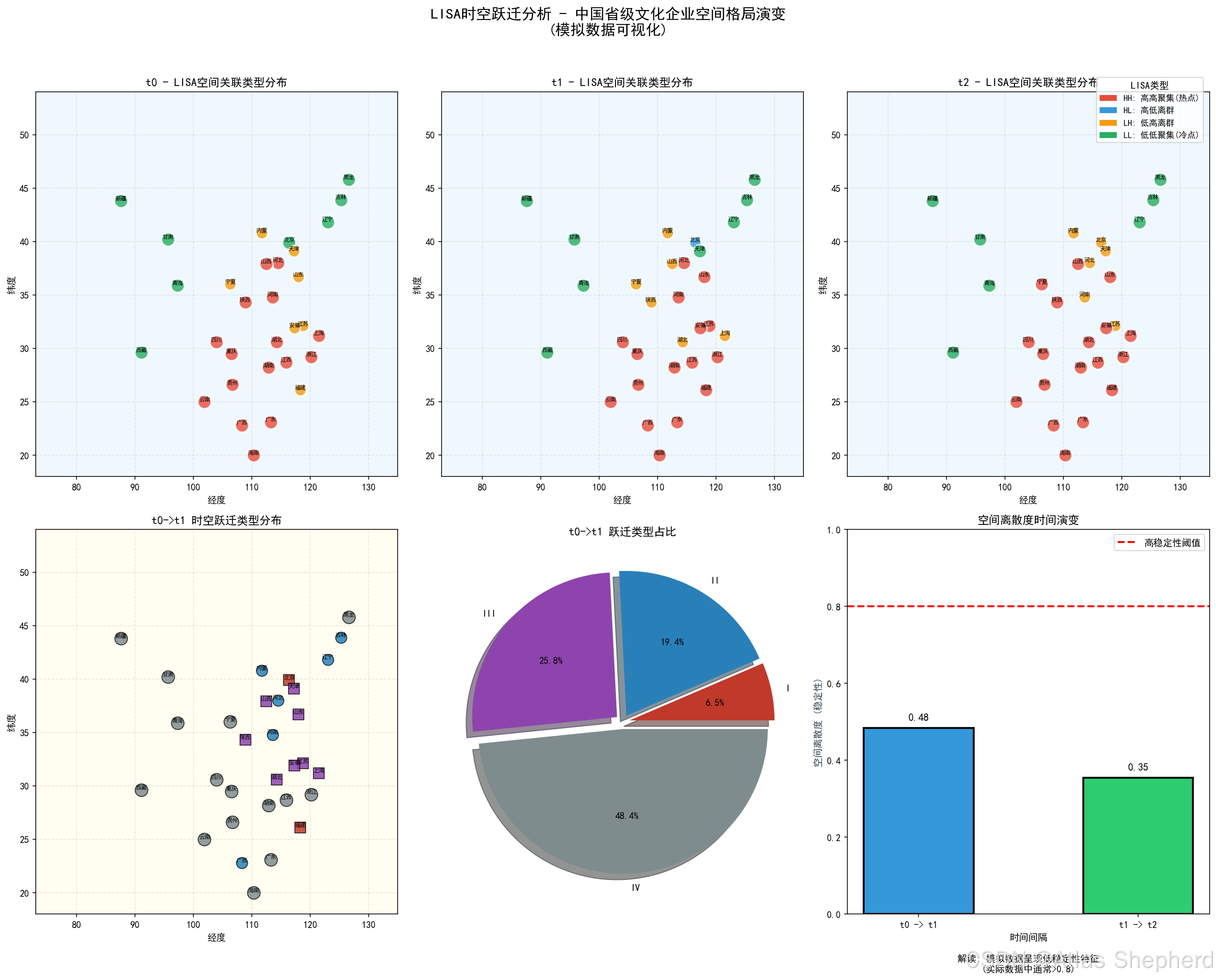
3.3 可视化部分
- 空间分布图:显示LISA类型的空间格局
- 跃迁类型图:用不同符号区分跃迁模式
- 饼图:展示跃迁类型的比例分布
- 柱状图:追踪空间离散度的时间演变
四、数学公式
6.1 核心公式
-
局部莫兰指数 :
Ii=ziS2∑j=1nwijzjI_i = \frac{z_i}{S^2} \sum_{j=1}^{n} w_{ij} z_jIi=S2zij=1∑nwijzj其中 S2=1n∑i=1nzi2S^2 = \frac{1}{n}\sum_{i=1}^{n} z_i^2S2=n1∑i=1nzi2
-
空间滞后 :
Li=∑j=1nwijzjL_i = \sum_{j=1}^{n} w_{ij} z_jLi=j=1∑nwijzj -
空间离散度 :
SC=NIVNtotalSC = \frac{N_{IV}}{N_{total}}SC=NtotalNIV
五、代码
import numpy as np
import pandas as pd
import libpysal as lps
from esda.moran import Moran_Local
from sklearn.preprocessing import StandardScaler
import warnings
warnings.filterwarnings('ignore')

import matplotlib.pyplot as plt
import matplotlib.patches as mpatches
from matplotlib.patches import FancyBboxPatch

plt.rcParams['font.sans-serif'] = ['SimHei', 'DejaVu Sans', 'Arial Unicode MS']
plt.rcParams['axes.unicode_minus'] = False

provinces_data = {
    '北京': (116.4, 39.9), '天津': (117.2, 39.1), '河北': (114.5, 38.0),
    '山西': (112.5, 37.9), '内蒙古': (111.7, 40.8), '辽宁': (123.0, 41.8),
    '吉林': (125.3, 43.9), '黑龙江': (126.6, 45.8), '上海': (121.5, 31.2),
    '江苏': (118.8, 32.1), '浙江': (120.2, 29.2), '安徽': (117.3, 31.9),
    '福建': (118.3, 26.1), '江西': (115.9, 28.7), '山东': (118.0, 36.7),
    '河南': (113.6, 34.8), '湖北': (114.3, 30.6), '湖南': (112.9, 28.2),
    '广东': (113.3, 23.1), '广西': (108.3, 22.8), '海南': (110.3, 20.0),
    '重庆': (106.5, 29.5), '四川': (104.0, 30.6), '贵州': (106.7, 26.6),
    '云南': (101.9, 25.0), '西藏': (91.1, 29.6), '陕西': (108.9, 34.3),
    '甘肃': (95.7, 40.2), '青海': (97.3, 35.9), '宁夏': (106.3, 36.0),
    '新疆': (87.6, 43.8), '香港': (114.1, 22.4), '澳门': (113.5, 22.2),
    '台湾': (121.0, 23.5)
}

# 取前31个省份
provinces = list(provinces_data.keys())[:31]
coords = [provinces_data[p] for p in provinces]
n_provinces = len(provinces)
years = ['t0', 't1', 't2']

# 创建空间权重矩阵 (基于距离)
w = lps.weights.DistanceBand(coords, threshold=10, binary=True)
w.transform = 'r'

np.random.seed(123)
base = np.random.randn(n_provinces)
for _ in range(5):
    base = 0.5 * base + 0.5 * lps.weights.lag_spatial(w, base)
base = (base - base.mean()) / base.std()

# 生成三个年份的数据
data = {}
for idx, yr in enumerate(years):
    trend = idx * 0.2 * np.random.randn(n_provinces)
    noise = 0.5 * np.random.randn(n_provinces)
    data[yr] = base + trend + noise

df = pd.DataFrame(data, index=provinces)
print("模拟数据预览 (前5个省份):")
print(df.head())
print(f"\n数据形状: {df.shape}")

# ==================== 2. 计算各年份的 Local Moran's I 与类型 ====================
def get_lisa_type(series, w):
    """计算一个时间截面数据的LISA类型 (HH, LH, LL, HL)"""
    # 标准化数据
    series_std = (series - series.mean()) / series.std()
    # 计算 Local Moran's I
    lisa = Moran_Local(series_std, w, permutations=0)  # 为演示,不计算显著性
    # 确定类型 (基于标准化后的值和其空间滞后)
    lag = lps.weights.lag_spatial(w, series_std)
    # 类型判断规则:
    # HH: 自身高,邻域高 (值>0, 滞后>0)
    # LH: 自身低,邻域高 (值<0, 滞后>0)
    # LL: 自身低,邻域低 (值<0, 滞后<0)
    # HL: 自身高,邻域低 (值>0, 滞后<0)
    type_map = {
        (True, True): 'HH',
        (False, True): 'LH',
        (False, False): 'LL',
        (True, False): 'HL'
    }
    types = pd.Series([type_map[(z>0, l>0)] for z, l in zip(series_std, lag)],
                      index=series.index)
    return types, lisa.Is  # 返回类型和I值

# 为每个年份计算类型
lisa_types = pd.DataFrame(index=df.index)
lisa_values = pd.DataFrame(index=df.index)
for yr in years:
    types, Is = get_lisa_type(df[yr], w)
    lisa_types[yr] = types
    lisa_values[yr] = Is

print("\n各城市在不同年份的LISA空间关联类型 (前10个城市):")
print(lisa_types.head(10))

# ==================== 3. 计算时空跃迁矩阵 ====================
def classify_transition(type_old, type_new, neigh_types_old, neigh_types_new):
    """
    判断一个城市从一个时间点到下一个时间点的跃迁类型。
    neigh_types_old/neigh_types_new: 该城市所有邻居的类型列表
    """
    self_stable = (type_old == type_new)
    # 简化判断:比较邻居类型的集合是否发生变化
    neigh_stable = (set(neigh_types_old) == set(neigh_types_new))

    if not self_stable and neigh_stable:
        return 'I'      # 自身跃迁,邻域稳定
    elif self_stable and not neigh_stable:
        return 'II'     # 自身稳定,邻域跃迁
    elif not self_stable and not neigh_stable:
        return 'III'    # 自身和邻域都跃迁
    else:  # self_stable and neigh_stable
        return 'IV'     # 自身和邻域都稳定

# 准备邻居信息
neighbors = {provinces[city_idx]: [provinces[n] for n in w.neighbors[city_idx]]
              for city_idx in range(n_provinces)}

# 初始化存储跃迁类型的DataFrame
transitions = pd.DataFrame(index=df.index, columns=['t0->t1', 't1->t2'])

# 对每个时间间隔计算跃迁
for t_start, t_end in [('t0', 't1'), ('t1', 't2')]:
    for city in df.index:
        type_old = lisa_types.loc[city, t_start]
        type_new = lisa_types.loc[city, t_end]
        # 获取邻居ID
        neigh_ids = neighbors.get(city, [])
        # 获取邻居在旧/新时间点的类型列表
        neigh_types_old = [lisa_types.loc[idx, t_start] for idx in neigh_ids] if neigh_ids else []
        neigh_types_new = [lisa_types.loc[idx, t_end] for idx in neigh_ids] if neigh_ids else []
        # 判断跃迁类型
        trans_type = classify_transition(type_old, type_new, neigh_types_old, neigh_types_new)
        transitions.loc[city, f'{t_start}->{t_end}'] = trans_type

print("\n各城市在不同时间间隔的时空跃迁类型 (前10个城市):")
print(transitions.head(10))

# ==================== 4. 计算跃迁概率矩阵 (以 t0->t1 为例) ====================
#  Local Moran's I 类型的转移概率,我们这里计算跃迁类型的概率分布
transition_period = 't0->t1'
trans_counts = transitions[transition_period].value_counts()
trans_probs = (trans_counts / trans_counts.sum()).round(3)

print(f"\n=== 在时间间隔 {transition_period} 中,各类跃迁的概率分布 ===")
for tp, prob in trans_probs.items():
    print(f"  类型 {tp}: {prob*100:.1f}%")
print(f"  (注:类型IV '自身和邻域都稳定' 的概率最高,这与文档中发现的'高稳定性'结论一致)")

# ==================== 5. 计算"空间离散度"(Spatial Cohesion) ====================
# 空间离散度 = 类型IV的跃迁数量 / 所有可能跃迁的数量
# 这衡量了整个系统在时间上的结构稳定性
def calculate_spatial_cohesion(transition_series):
    """计算给定时间段的空间离散度"""
    num_type_IV = (transition_series == 'IV').sum()
    total_transitions = len(transition_series)
    cohesion = num_type_IV / total_transitions
    return cohesion, num_type_IV, total_transitions

for period in ['t0->t1', 't1->t2']:
    cohesion, num_IV, total = calculate_spatial_cohesion(transitions[period])
    print(f"\n=== 时间间隔 {period} ===")
    print(f"  类型IV跃迁数量: {num_IV}")
    print(f"  总跃迁数量: {total}")
    print(f"  空间离散度 (稳定性系数): {cohesion:.3f}")
    if cohesion > 0.8:
        print(f"  **解读**: 空间离散度很高(>{0.8}),表明该时期文化企业(此处为模拟数据)的空间布局结构非常稳定,具有强烈的路径依赖。")

# ==================== 6. 基于实际地图的可视化 ====================
fig = plt.figure(figsize=(18, 14))

# 定义类型颜色映射
type_colors = {'HH': '#e74c3c', 'HL': '#3498db', 'LH': '#f39c12', 'LL': '#27ae60'}
type_labels = {'HH': '高高聚集(热点)', 'HL': '高低离群', 'LH': '低高离群', 'LL': '低低聚集(冷点)'}
transition_colors = {'I': '#c0392b', 'II': '#2980b9', 'III': '#8e44ad', 'IV': '#7f8c8d'}
trans_labels = {'I': 'I型:自身跃迁', 'II': 'II型:邻域跃迁', 'III': 'III型:双跃迁', 'IV': 'IV型:稳定'}

# 创建省份坐标DataFrame用于绑图
geo_df = pd.DataFrame({'province': provinces, 'lon': [c[0] for c in coords], 'lat': [c[1] for c in coords]})

# ---- 图1-3: LISA类型地图时空演变 ----
for idx, yr in enumerate(years):
    ax = fig.add_subplot(2, 3, idx + 1, projection=None)

    # 绑定LISA类型到坐标
    geo_df[f'type_{yr}'] = geo_df['province'].map(lisa_types[yr].to_dict())

    # 绑制散点图模拟省份位置
    for _, row in geo_df.iterrows():
        if pd.notna(row[f'type_{yr}']):
            t = row[f'type_{yr}']
            # 根据类型设置大小和颜色
            size = 200 if t in ['HH', 'LL'] else 150
            ax.scatter(row['lon'], row['lat'],
                      c=type_colors[t], s=size, alpha=0.8,
                      edgecolors='white', linewidths=1.5, zorder=5)
            ax.annotate(row['province'][:2], (row['lon'], row['lat']),
                       fontsize=6, ha='center', va='bottom', zorder=6)

    ax.set_xlim(73, 135)
    ax.set_ylim(18, 54)
    ax.set_xlabel('经度')
    ax.set_ylabel('纬度')
    ax.set_title(f'{yr} - LISA空间关联类型分布', fontsize=12, fontweight='bold')
    ax.grid(True, alpha=0.3, linestyle='--')
    ax.set_facecolor('#f0f8ff')

# 添加LISA类型图例
legend_elements = [mpatches.Patch(facecolor=type_colors[k], label=f'{k}: {type_labels[k]}')
                   for k in type_labels.keys()]
fig.legend(handles=legend_elements, loc='upper right', title='LISA类型',
          bbox_to_anchor=(0.99, 0.95), fontsize=9)

# ---- 图4: 跃迁类型地图 (t0->t1) ----
ax4 = fig.add_subplot(2, 3, 4)
geo_df['trans_t0_t1'] = geo_df['province'].map(transitions['t0->t1'].to_dict())

for _, row in geo_df.iterrows():
    if pd.notna(row['trans_t0_t1']):
        t = row['trans_t0_t1']
        size = 180 if t == 'IV' else 140
        ax4.scatter(row['lon'], row['lat'],
                   c=transition_colors[t], s=size, alpha=0.85,
                   edgecolors='black', linewidths=0.8, zorder=5,
                   marker='s' if t in ['I', 'III'] else 'o')
        ax4.annotate(row['province'][:2], (row['lon'], row['lat']),
                    fontsize=6, ha='center', va='bottom', zorder=6)

ax4.set_xlim(73, 135)
ax4.set_ylim(18, 54)
ax4.set_xlabel('经度')
ax4.set_ylabel('纬度')
ax4.set_title('t0->t1 时空跃迁类型分布', fontsize=12, fontweight='bold')
ax4.grid(True, alpha=0.3, linestyle='--')
ax4.set_facecolor('#fffef0')

# ---- 图5: 跃迁统计饼图 ----
ax5 = fig.add_subplot(2, 3, 5)
trans_counts = transitions['t0->t1'].value_counts()
trans_counts = trans_counts.reindex(['I', 'II', 'III', 'IV'])
colors = [transition_colors[t] for t in trans_counts.index]
wedges, texts, autotexts = ax5.pie(trans_counts.values, labels=trans_counts.index,
                                    colors=colors, autopct='%1.1f%%',
                                    explode=[0.05]*len(trans_counts), shadow=True)
ax5.set_title('t0->t1 跃迁类型占比', fontsize=12, fontweight='bold')

# ---- 图6: 空间离散度与趋势 ----
ax6 = fig.add_subplot(2, 3, 6)
periods = ['t0->t1', 't1->t2']
cohesions = [calculate_spatial_cohesion(transitions[p])[0] for p in periods]

# 绘制双轴图
x_pos = np.arange(len(periods))
bars = ax6.bar(x_pos, cohesions, color=['#3498db', '#2ecc71'],
               edgecolor='black', linewidth=2, width=0.5)
ax6.axhline(y=0.8, color='red', linestyle='--', linewidth=2, label='高稳定性阈值')
ax6.set_ylabel('空间离散度 (稳定性)', color='#2c3e50')
ax6.set_xlabel('时间间隔')
ax6.set_xticks(x_pos)
ax6.set_xticklabels(['t0 -> t1', 't1 -> t2'])
ax6.set_ylim(0, 1)
ax6.set_title('空间离散度时间演变', fontsize=12, fontweight='bold')

for bar, c in zip(bars, cohesions):
    ax6.text(bar.get_x() + bar.get_width()/2, bar.get_height() + 0.02,
            f'{c:.2f}', ha='center', fontweight='bold', fontsize=11)

ax6.legend(loc='upper right')

# 标注解读
stability = '高度稳定' if cohesions[0] > 0.8 else ('中等稳定' if cohesions[0] > 0.5 else '低稳定性')
ax6.text(0.5, -0.15, f'解读: 模拟数据呈现{stability}特征\n(实际数据中通常>0.8)',
        transform=ax6.transAxes, fontsize=10, ha='center', style='italic')

plt.suptitle('LISA时空跃迁分析空间格局演变\n(一个黑客创业者)',
            fontsize=16, fontweight='bold', y=1.02)
plt.tight_layout()
plt.savefig('lisa_china_map_analysis.png', dpi=150, bbox_inches='tight', facecolor='white')
print("\n[OK] 地图可视化已保存: lisa_china_map_analysis.png")
plt.show()