学习率调度------让学习"先快后慢"
📚 《从零到一造大脑:AI架构入门之旅》专栏
专栏定位 :面向中学生、大学生和 AI 初学者的科普专栏,用大白话和生活化比喻带你从零理解人工智能
本系列共 43 篇,分为八大模块:
- 📖 模块一【AI 基础概念】(3 篇):AI/ML/DL 关系、学习方式、深度之谜
- 🧠 模块二【神经网络入门】(4 篇):神经元、权重、激活函数、MLP
- 🏗️ 模块三【深度学习核心】(6 篇):损失函数、梯度下降、反向传播、过拟合、Batch/Epoch/LR
- 🎯 模块四【注意力机制】(5 篇):从 Attention 到 Transformer
- 🔬 模块五【NCT 与 CATS-NET 案例】(8 篇):真实架构演进全记录
- 🔄 模块六【架构融合方法】(6 篇):如何设计混合架构
- ⚙️ 模块七【调参炼丹术】(7 篇):学习率、正则化、超参数搜索
- 🚀 模块八【综合应用展望】(4 篇):未来趋势与职业规划
本文是模块七第 5 篇,带你理解学习率调度的核心策略。👨💻 作者简介:NeuroConscious Research Team,一群热爱 AI 科普的研究者,专注于神经科学启发的 AI架构设计与可解释性研究。理念:"再复杂的概念,也能用大白话讲清楚"。
💻 项目地址 :https://github.com/wyg5208/nct.git
🌐 官网地址 :https://neuroconscious.link
📝 作者 CSDN :https://blog.csdn.net/yweng18
📦 NCT PyPI :https://pypi.org/project/neuroconscious-transformer/
⭐ 欢迎 Star⭐、Fork🍴、贡献代码🤝
📌 本文核心比喻 :马拉松配速策略
⏱️ 阅读时间 :约 20 分钟
🎯 学习目标:理解为什么需要学习率调度,掌握常见调度策略的使用场景
📝 文章摘要
学习率调度是深度学习训练中的"配速策略"。就像跑马拉松不能全程冲刺一样,训练神经网络也需要在前期大步快跑、后期小步微调。本文介绍 Step Decay、Cosine Annealing、Warmup+Decay、ReduceLROnPlateau 等常见策略,帮你在不同场景下选择最合适的"配速方案"。
🎯 你需要先了解
阅读本文前,建议你:
- ✅ 理解学习率的概念(参考第 10 篇)
- ✅ 知道梯度下降的基本原理
- ✅ 了解训练过程中的 Loss 曲线
如果还没读前文,点这里返回(40-权重衰减 L2正则化实战_version_B.md)
📖 正文
一、为什么需要学习率调度?
1.1 训练过程中的"配速"问题
🏃 马拉松配速的智慧
跑马拉松的老手都知道:
起跑阶段 :体力充沛,可以跑快一点
中途阶段 :保持节奏,稳定配速
冲刺阶段 :接近终点,需要精细控制
如果全程用冲刺速度? → 很快就累垮了
如果全程用慢跑速度? → 永远跑不到终点
1.2 学习率的"配速"困境
训练神经网络和跑马拉松有惊人的相似之处:
| 训练阶段 | 参数状态 | 需要的学习率 | 类比 |
|---|---|---|---|
| 初期 | 离最优解很远 | 大(大步快走) | 高速公路,油门踩大 |
| 中期 | 逐渐接近 | 中等 | 市区道路,适度减速 |
| 后期 | 接近最优解 | 小(小步微调) | 进站停车,轻踩刹车 |
⚠️ 固定学习率的问题
学习率太大 :
• 训练后期在最优解附近震荡
• 无法收敛到精确的最小值
• Loss 曲线剧烈抖动
学习率太小 :
• 训练初期进展极慢
• 可能陷入局部最优
• 需要非常多的 epoch 才能收敛
1.3 学习率调度的核心思想
学习率调度的核心思想
训练初期:大学习率
- 参数离最优解远,需要"大步快走"
- 快速逼近最优解附近区域
训练后期:小学习率
- 参数已接近最优解,需要"小步微调"
- 精确定位最优解
类比:射箭
- 第一阶段:粗略瞄准(大学习率)
- 第二阶段:精细调整(小学习率)
二、常见学习率调度策略
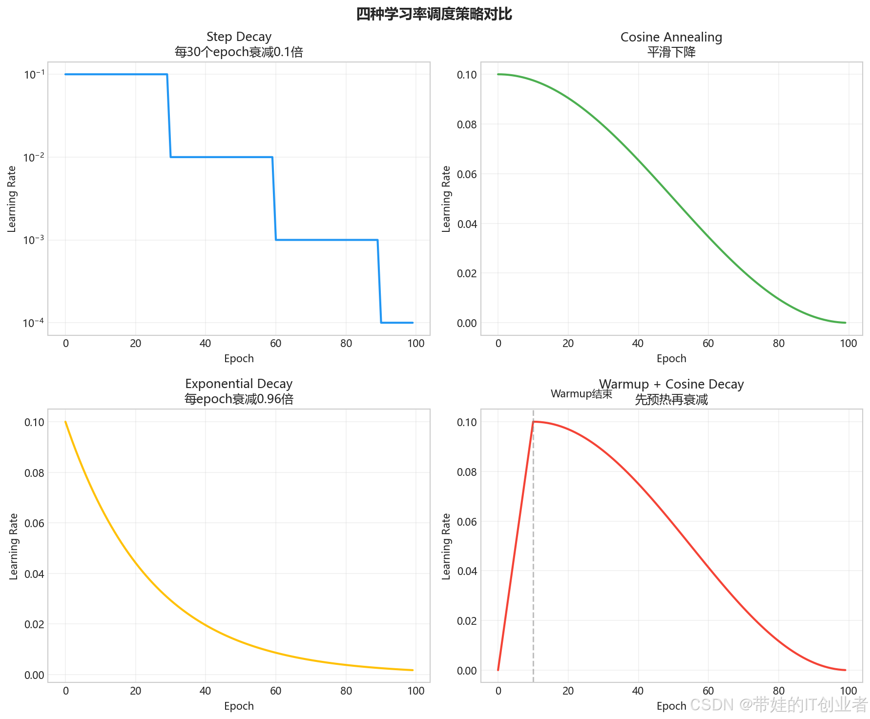
2.1 Step Decay(阶梯下降)
📉 阶梯下降策略
核心思想 :每隔固定的 epoch 数,学习率乘以一个衰减因子
生活类比 :阶梯电价
• 第一档电量:单价高
• 超过一定度数:降到第二档
• 再超过:降到第三档
python
from torch.optim.lr_scheduler import StepLR
import torch.optim as optim
import matplotlib.pyplot as plt

# 定义模型和优化器
model = ...  # 你的模型
optimizer = optim.SGD(model.parameters(), lr=0.1)

# Step Decay 调度器
# 每 30 个 epoch,学习率乘以 0.1
scheduler = StepLR(optimizer, step_size=30, gamma=0.1)

# 训练循环
learning_rates = []
for epoch in range(100):
    # 训练代码...
    train_one_epoch(...)

    # 更新学习率
    scheduler.step()
    learning_rates.append(optimizer.param_groups[0]['lr'])

# 可视化学习率变化
plt.figure(figsize=(10, 5))
plt.plot(learning_rates, linewidth=2)
plt.xlabel('Epoch')
plt.ylabel('Learning Rate')
plt.title('Step Decay: step_size=30, gamma=0.1')
plt.grid(True, alpha=0.3)
plt.savefig('img_41_step_decay.png', dpi=150, bbox_inches='tight')
plt.show()
Step Decay 的学习率变化:
Epoch 0-29:   LR = 0.1   (初始学习率)
Epoch 30-59:  LR = 0.01  (衰减一次)
Epoch 60-89:  LR = 0.001 (衰减两次)
Epoch 90-99:  LR = 0.0001(衰减三次)
2.2 Exponential Decay(指数衰减)
📊 指数衰减策略
核心思想 :每个 epoch 学习率都按指数衰减
数学公式 :lr = lr_init × γ^epoch
生活类比 :手机电池电量
• 每小时剩余电量的百分比相同
• 形成平滑的衰减曲线
python
from torch.optim.lr_scheduler import ExponentialLR

# Exponential Decay 调度器
# 每个 epoch,学习率乘以 0.99
scheduler = ExponentialLR(optimizer, gamma=0.99)

# 学习率变化:
# Epoch 0:   LR = 0.1 × 0.99^0  = 0.1
# Epoch 10:  LR = 0.1 × 0.99^10 ≈ 0.090
# Epoch 50:  LR = 0.1 × 0.99^50 ≈ 0.606
# Epoch 100: LR = 0.1 × 0.99^100 ≈ 0.366
2.3 Cosine Annealing(余弦退火)
🌊 余弦退火策略
核心思想 :学习率按余弦曲线从大到小变化
生活类比 :滑滑梯
• 开始时下降平缓(高学习率保持一段时间)
• 中间下降加速
• 最后平缓落地(低学习率保持一段时间)
python
from torch.optim.lr_scheduler import CosineAnnealingLR

# Cosine Annealing 调度器
# T_max: 一个周期的 epoch 数
# eta_min: 最小学习率
scheduler = CosineAnnealingLR(optimizer, T_max=100, eta_min=1e-6)

# 学习率公式:
# lr = eta_min + 0.5 * (lr_init - eta_min) * (1 + cos(π * epoch / T_max))
**Cosine Annealing 的特点**:

<div style="background-color: #e8f5e9; padding: 20px; border-radius: 8px; border-left: 4px solid #4caf50;">

### Cosine Annealing 特点

**优点:**
- ✓ 平滑下降,无突变
- ✓ 训练后期学习率很小,有利于精细调优
- ✓ 在大模型训练中效果优秀

**适用场景:**
- 大规模模型训练
- 需要平滑收敛的任务
- 计算机视觉、NLP 等

</div>

#### 2.4 Warmup + Decay(预热+衰减)

<div style="background-color: #e0f2f1; padding: 15px; border-left: 4px solid #009688; border-radius: 5px;">
<strong>🔥 预热策略</strong><br><br>

<strong>核心思想</strong>:先让学习率从 0 线性增加到目标值,再开始衰减<br><br>

<strong>为什么需要 Warmup?</strong><br>
• 训练开始时参数是随机的,直接用大学习率可能导致梯度爆炸<br>
• Warmup 让模型"热身",稳定后再加速<br><br>

<strong>生活类比</strong>:冬天开车<br>
• 启动前先热车(Warmup)<br>
• 水温正常后再加速(大学习率)<br>
• 接近目的地减速(衰减)
</div>

```python
from torch.optim.lr_scheduler import LambdaLR
import math

def warmup_cosine_schedule(epoch, warmup_epochs=10, total_epochs=100):
    """
    Warmup + Cosine Decay 学习率调度
    """
    if epoch < warmup_epochs:
        # Warmup 阶段:线性增加
        return epoch / warmup_epochs
    else:
        # Cosine Decay 阶段
        progress = (epoch - warmup_epochs) / (total_epochs - warmup_epochs)
        return 0.5 * (1 + math.cos(math.pi * progress))

# 创建调度器
scheduler = LambdaLR(
    optimizer,
    lr_lambda=lambda epoch: warmup_cosine_schedule(epoch, warmup_epochs=10, total_epochs=100)
)
Warmup + Cosine 的学习率变化:
学习率变化曲线:

LR ▲
    │    ╭──────╮
    │   ╱        ╲
    │  ╱          ╲
    │ ╱            ╲
    │╱              ╲
    └──────────────────────▶ Epoch
    0  10           100

    ↑               ↑
  Warmup         Cosine
  阶段           Decay
2.5 ReduceLROnPlateau(自适应衰减)
🎯 自适应衰减策略
核心思想 :当指标(如 Loss)不再改善时,自动降低学习率
生活类比 :智能空调
• 温度稳定时保持当前档位
• 温度长时间不变时自动调低
• 检测到温度波动时重新调整
python
from torch.optim.lr_scheduler import ReduceLROnPlateau

# ReduceLROnPlateau 调度器
scheduler = ReduceLROnPlateau(
    optimizer,
    mode='min',          # 监控指标越小越好
    factor=0.1,          # 衰减因子
    patience=10,         # 10 个 epoch 没改善就衰减
    verbose=True,        # 打印调整信息
    min_lr=1e-6          # 最小学习率
)

# 训练循环
for epoch in range(100):
    train_loss = train_one_epoch(...)
    val_loss = validate(...)

    # 根据验证集 Loss 调整学习率
    scheduler.step(val_loss)
**ReduceLROnPlateau 的优势**:

<div style="background-color: #fff3e0; padding: 20px; border-radius: 8px; border-left: 4px solid #ff9800;">

### ReduceLROnPlateau 特点

**优点:**
- ✓ 无需预设衰减时机
- ✓ 自动根据训练情况调整
- ✓ 适合不知道需要多少 epoch 的任务

**缺点:**
- ✗ 需要额外监控指标
- ✗ 可能错过最优衰减时机

**适用场景:**
- 不确定训练需要多久
- 需要根据验证集表现调整

</div>

---

### 三、调度策略大比拼

#### 3.1 四种策略可视化对比

```python
import torch
import torch.optim as optim
from torch.optim.lr_scheduler import (
    StepLR, ExponentialLR, CosineAnnealingLR, ReduceLROnPlateau
)
import matplotlib.pyplot as plt
import numpy as np

# 模拟一个简单模型
model = torch.nn.Linear(10, 1)
optimizer = optim.SGD(model.parameters(), lr=0.1)

# 创建不同的调度器
schedulers = {
    'Step (step=30, γ=0.1)': StepLR(optimizer, step_size=30, gamma=0.1),
    'Exponential (γ=0.99)': ExponentialLR(optimizer, gamma=0.99),
    'Cosine (T_max=100)': CosineAnnealingLR(optimizer, T_max=100, eta_min=1e-6),
}

# 记录学习率
lr_history = {name: [] for name in schedulers}

# 模拟训练
for epoch in range(100):
    for name, scheduler in schedulers.items():
        lr_history[name].append(optimizer.param_groups[0]['lr'])
        scheduler.step()

# 绘制对比图
fig, axes = plt.subplots(1, 3, figsize=(15, 5))

for idx, (name, lrs) in enumerate(lr_history.items()):
    axes[idx].plot(lrs, linewidth=2, color=f'C{idx}')
    axes[idx].set_xlabel('Epoch')
    axes[idx].set_ylabel('Learning Rate')
    axes[idx].set_title(name)
    axes[idx].grid(True, alpha=0.3)
    axes[idx].set_yscale('log')

plt.tight_layout()
plt.savefig('img_41_scheduler_comparison.png', dpi=150, bbox_inches='tight')
plt.show()
3.2 策略选择指南
| 策略 | 特点 | 适用场景 | 参数 |
|---|---|---|---|
| Step Decay | 简单直观,阶梯式下降 | 简单任务、快速实验 | step_size, gamma |
| Exponential | 平滑衰减,每个 epoch 都变 | 需要持续衰减的任务 | gamma |
| Cosine | 平滑下降,后期稳定 | 大模型训练、CV/NLP | T_max, eta_min |
| Warmup+Cosine | 预热+衰减,稳定性好 | Transformer、大模型 | warmup_epochs |
| ReduceLROnPlateau | 自适应,按需调整 | 不确定训练时长的任务 | patience, factor |
| OneCycleLR | 自动规划整个训练过程 | 快速训练、AutoML | max_lr, total_steps |
💡 选择建议
新手推荐 :Step Decay 或 Cosine Annealing
大模型推荐 :Warmup + Cosine
不确定训练时长 :ReduceLROnPlateau
追求最高效训练:OneCycleLR
四、OneCycleLR:一站式解决方案
🚀 OneCycleLR 策略
核心思想 :用一个周期完成学习率的"升温-保持-降温"全过程
发明者 :Leslie Smith (2017)
特点 :
• 自动规划整个训练过程的学习率
• 先升后降,中间可能有个峰值
• 被证明在很多任务上效果很好
python
from torch.optim.lr_scheduler import OneCycleLR

# OneCycleLR 调度器
scheduler = OneCycleLR(
    optimizer,
    max_lr=0.1,           # 最大学习率
    total_steps=1000,     # 总步数(epochs × batches_per_epoch)
    pct_start=0.3,        # 升温阶段占比 30%
    anneal_strategy='cos', # 使用余弦衰减
    div_factor=25,        # 初始学习率 = max_lr / 25
    final_div_factor=1e4  # 最终学习率 = max_lr / 10000
)

# OneCycleLR 需要在每个 batch 后调用,而不是每个 epoch
for epoch in range(100):
    for batch_idx, (data, target) in enumerate(train_loader):
        # 前向传播
        output = model(data)
        loss = criterion(output, target)

        # 反向传播
        optimizer.zero_grad()
        loss.backward()
        optimizer.step()

        # 更新学习率(每个 batch)
        scheduler.step()
OneCycleLR 的学习率曲线:
学习率变化:

LR ▲
    │        ╭──╮
    │       ╱    ╲
    │      ╱      ╲
    │     ╱        ╲
    │    ╱          ╲
    │   ╱            ╲
    │──╯              ╲───
    └──────────────────────▶ Steps
    0    30%          100%

    ↑    ↑            ↑
  起步  峰值        结束
五、在 PyTorch 中使用学习率调度
5.1 完整训练示例
python
import torch
import torch.nn as nn
import torch.optim as optim
from torch.optim.lr_scheduler import CosineAnnealingLR
import matplotlib.pyplot as plt

# 1. 定义模型
class SimpleModel(nn.Module):
    def __init__(self):
        super().__init__()
        self.fc1 = nn.Linear(784, 256)
        self.fc2 = nn.Linear(256, 128)
        self.fc3 = nn.Linear(128, 10)
        self.relu = nn.ReLU()

    def forward(self, x):
        x = x.view(-1, 784)
        x = self.relu(self.fc1(x))
        x = self.relu(self.fc2(x))
        return self.fc3(x)

model = SimpleModel()

# 2. 定义优化器和调度器
optimizer = optim.Adam(model.parameters(), lr=0.01)
scheduler = CosineAnnealingLR(optimizer, T_max=50, eta_min=1e-6)

# 3. 训练循环
train_losses = []
learning_rates = []

for epoch in range(50):
    # 训练一个 epoch
    model.train()
    epoch_loss = 0.0

    for batch_idx, (data, target) in enumerate(train_loader):
        optimizer.zero_grad()
        output = model(data)
        loss = nn.CrossEntropyLoss()(output, target)
        loss.backward()
        optimizer.step()
        epoch_loss += loss.item()

    # 更新学习率
    scheduler.step()

    # 记录
    avg_loss = epoch_loss / len(train_loader)
    train_losses.append(avg_loss)
    learning_rates.append(optimizer.param_groups[0]['lr'])

    print(f"Epoch {epoch+1}: Loss = {avg_loss:.4f}, LR = {learning_rates[-1]:.6f}")

# 4. 可视化
fig, (ax1, ax2) = plt.subplots(1, 2, figsize=(12, 5))

ax1.plot(train_losses, 'b-', linewidth=2)
ax1.set_xlabel('Epoch')
ax1.set_ylabel('Training Loss')
ax1.set_title('Loss vs Epoch')
ax1.grid(True, alpha=0.3)

ax2.plot(learning_rates, 'r-', linewidth=2)
ax2.set_xlabel('Epoch')
ax2.set_ylabel('Learning Rate')
ax2.set_title('Learning Rate Schedule (Cosine)')
ax2.grid(True, alpha=0.3)

plt.tight_layout()
plt.savefig('img_41_training_with_scheduler.png', dpi=150, bbox_inches='tight')
plt.show()
5.2 关键注意事项
⚠️ 常见错误
错误 1:scheduler.step() 位置不对
python
# ❌ 错误:在 optimizer.step() 之前调用
scheduler.step()
optimizer.step()

# ✅ 正确:在 optimizer.step() 之后调用
optimizer.step()
scheduler.step()
错误 2:OneCycleLR 在 epoch 结束时调用
python
# ❌ 错误:OneCycleLR 应该在 batch 级别调用
for epoch in range(epochs):
    train_one_epoch()
    scheduler.step()  # 这样不对

# ✅ 正确:在每个 batch 后调用
for epoch in range(epochs):
    for batch in train_loader:
        optimizer.step()
        scheduler.step()  # 正确!
错误 3:忘记传递监控指标给 ReduceLROnPlateau
python
# ❌ 错误:ReduceLROnPlateau 需要监控指标
scheduler.step()

# ✅ 正确:传入验证集 Loss
val_loss = validate()
scheduler.step(val_loss)
六、NCT 中的学习率调度
python
# NCT 项目中使用的学习率调度配置
from torch.optim.lr_scheduler import CosineAnnealingWarmRestarts

def get_scheduler(optimizer, config):
    """
    NCT 默认使用 Cosine Annealing with Warmup

    为什么选择这个?
    1. 概念模块:Cosine + Warmup 保持稳定
    2. 全局工作空间:继承预训练,用小学习率微调
    3. 整体训练:平滑收敛,避免震荡
    """

    def lr_lambda(epoch):
        # Warmup 阶段
        if epoch < config.warmup_epochs:
            return epoch / config.warmup_epochs
        # Cosine Decay 阶段
        else:
            progress = (epoch - config.warmup_epochs) / (config.total_epochs - config.warmup_epochs)
            return 0.5 * (1 + math.cos(math.pi * progress))

    return LambdaLR(optimizer, lr_lambda)

# 使用示例
config = {
    'warmup_epochs': 5,
    'total_epochs': 100,
}

scheduler = get_scheduler(optimizer, config)
⚠️ 常见误区
⚠️ 误区警示区
❌ 误区 1:"学习率衰减越快越好"
真相:
学习率衰减太快会导致过早陷入局部最优,无法充分探索参数空间。衰减太慢则训练后期效率低下。需要根据任务特点选择合适的衰减速度。
❌ 误区 2:"Warmup 只是大模型需要"
真相:
虽然 Warmup 对大模型(如 Transformer)特别重要,但小模型也可能受益。特别是当初始参数是随机初始化时,Warmup 可以帮助稳定训练初期。
❌ 误区 3:"调度器可以解决所有学习率问题"
真相:
调度器只是辅助工具,选择合适的初始学习率仍然是最重要的。如果初始学习率设置不当,再好的调度器也无法挽救。
💡 一句话总结
🎯 核心结论
学习率调度 = 训练的"配速策略"
前期大步快走,后期小步微调,让模型既跑得快,又站得稳。
记忆口诀:
学习率,要调度,
先大后小是妙招。
Step 简单 Cosine 平,
Warmup 护航大模型。
ReduceLROnPlateau 最智能,
看 Loss 不动才衰减。
🔬 动手实验
实验:可视化不同调度策略的效果
python
"""
实验目标:对比不同学习率调度策略对训练的影响
"""
import torch
import torch.nn as nn
import torch.optim as optim
from torch.optim.lr_scheduler import StepLR, CosineAnnealingLR, OneCycleLR
import matplotlib.pyplot as plt
from torchvision import datasets, transforms

# 准备数据
transform = transforms.Compose([
    transforms.ToTensor(),
    transforms.Normalize((0.1307,), (0.3081,))
])

train_dataset = datasets.MNIST('./data', train=True, download=True, transform=transform)
train_loader = torch.utils.data.DataLoader(train_dataset, batch_size=64, shuffle=True)

# 定义模型
def create_model():
    return nn.Sequential(
        nn.Flatten(),
        nn.Linear(784, 128),
        nn.ReLU(),
        nn.Linear(128, 10)
    )

# 训练函数
def train_with_scheduler(scheduler_name, scheduler_fn, epochs=10):
    model = create_model()
    optimizer = optim.Adam(model.parameters(), lr=0.01)
    scheduler = scheduler_fn(optimizer)

    losses = []
    lrs = []

    for epoch in range(epochs):
        model.train()
        epoch_loss = 0.0

        for data, target in train_loader:
            optimizer.zero_grad()
            output = model(data)
            loss = nn.CrossEntropyLoss()(output, target)
            loss.backward()
            optimizer.step()

            # OneCycleLR 需要每个 batch 调用
            if scheduler_name == 'OneCycleLR':
                scheduler.step()

            epoch_loss += loss.item()

        # 其他调度器每个 epoch 调用
        if scheduler_name != 'OneCycleLR':
            scheduler.step()

        losses.append(epoch_loss / len(train_loader))
        lrs.append(optimizer.param_groups[0]['lr'])

    return losses, lrs

# 运行实验
schedulers = {
    'StepLR': lambda opt: StepLR(opt, step_size=3, gamma=0.5),
    'Cosine': lambda opt: CosineAnnealingLR(opt, T_max=10, eta_min=1e-5),
    'OneCycleLR': lambda opt: OneCycleLR(opt, max_lr=0.01, total_steps=10*len(train_loader)),
}

results = {}
for name, fn in schedulers.items():
    print(f"Training with {name}...")
    results[name] = train_with_scheduler(name, fn)

# 可视化结果
fig, axes = plt.subplots(1, 2, figsize=(14, 5))

for name, (losses, lrs) in results.items():
    axes[0].plot(losses, label=name, linewidth=2)
    axes[1].plot(lrs, label=name, linewidth=2)

axes[0].set_xlabel('Epoch')
axes[0].set_ylabel('Training Loss')
axes[0].set_title('Loss Comparison')
axes[0].legend()
axes[0].grid(True, alpha=0.3)

axes[1].set_xlabel('Epoch')
axes[1].set_ylabel('Learning Rate')
axes[1].set_title('Learning Rate Schedule')
axes[1].legend()
axes[1].grid(True, alpha=0.3)

plt.tight_layout()
plt.savefig('img_41_experiment_comparison.png', dpi=150, bbox_inches='tight')
plt.show()

print("实验完成!对比不同调度策略的效果。")
📚 延伸阅读
- PyTorch 官方文档:LR Scheduler
- SGDR: Stochastic Gradient Descent with Warm Restarts
- Super-Convergence: One Cycle Learning Rate
- AdamW 和学习率调度
✍️ 课后作业
选择题(每题 10 分)
1. Step Decay 调度策略的特点是?
A. 学习率平滑下降
B. 学习率按阶梯状下降 ✅
C. 学习率先升后降
D. 学习率自适应调整
2. 为什么 Transformer 训练时常用 Warmup?
A. 为了让训练更慢
B. 为了防止训练初期梯度不稳定 ✅
C. 为了增加学习率
D. 为了减少参数数量
3. OneCycleLR 调度器应该在什么时候调用?
A. 每个 epoch 开始时
B. 每个 epoch 结束时
C. 每个 batch 结束后 ✅
D. 训练完成后
思考题(20 分)
实验:在你之前的训练代码中,尝试添加 Cosine Annealing 调度器,对比固定学习率和动态调度的效果差异。记录 Loss 曲线的变化。
📝 下一篇预告
🚀 下一篇文章
题目 :实战:MNIST 上调参全流程演示
我们会学到:
- 完整的调参流程:从基线到最优
- 学习率、Batch Size、正则化的协同调整
- 如何记录和分析实验结果
📌 本文属《从零到一造大脑:AI架构入门之旅》专栏第七模块第五篇
作者:NeuroConscious Research Team
更新时间:2026 年 4 月
版本号:V1.0(图文并茂版)