ResNet-50学习笔记

• 🍨 本文为🔗365天深度学习训练营 中的学习记录博客
• 🍖 原作者：K同学啊

一、前期准备

import matplotlib.pyplot as plt
import numpy as np
import tensorflow as tf
from tensorflow.keras import layers, models, Input

# 1. 设置 GPU 环境
gpus = tf.config.list_physical_devices('GPU')
print("Found GPUs:", gpus)

# 2. 导入数据
data_dir = './J1_data' 
img_height = 224
img_width = 224
batch_size = 32

train_ds = tf.keras.utils.image_dataset_from_directory(
    data_dir,
    validation_split=0.2,
    subset="training",
    seed=123,
    image_size=(img_height, img_width),
    batch_size=batch_size)

val_ds = tf.keras.utils.image_dataset_from_directory(
    data_dir,
    validation_split=0.2,
    subset="validation",
    seed=123,
    image_size=(img_height, img_width),
    batch_size=batch_size)

class_names = train_ds.class_names
print(f"识别目标类别: {class_names}")

AUTOTUNE = tf.data.AUTOTUNE
train_ds = train_ds.cache().shuffle(1000).prefetch(buffer_size=AUTOTUNE)
val_ds = val_ds.cache().prefetch(buffer_size=AUTOTUNE)

二、核心：构建 ResNet 的残差块

# 2.1 恒等块 (Identity Block) - 输入输出维度一致时使用
def identity_block(input_tensor, kernel_size, filters):
    filters1, filters2, filters3 = filters
    
    # 主路径
    x = layers.Conv2D(filters1, (1, 1))(input_tensor)
    x = layers.BatchNormalization()(x)
    x = layers.Activation('relu')(x)
    
    x = layers.Conv2D(filters2, kernel_size, padding='same')(x)
    x = layers.BatchNormalization()(x)
    x = layers.Activation('relu')(x)
    
    x = layers.Conv2D(filters3, (1, 1))(x)
    x = layers.BatchNormalization()(x)
    
    # 核心：抄近道（Skip Connection），将输入直接加到输出上
    x = layers.add([x, input_tensor])
    x = layers.Activation('relu')(x)
    return x

# 2.2 卷积块 (Conv Block) - 输入输出维度不一致时使用，近道上也加个卷积核调整维度
def conv_block(input_tensor, kernel_size, filters, strides=(2, 2)):
    filters1, filters2, filters3 = filters
    
    # 主路径
    x = layers.Conv2D(filters1, (1, 1), strides=strides)(input_tensor)
    x = layers.BatchNormalization()(x)
    x = layers.Activation('relu')(x)
    
    x = layers.Conv2D(filters2, kernel_size, padding='same')(x)
    x = layers.BatchNormalization()(x)
    x = layers.Activation('relu')(x)
    
    x = layers.Conv2D(filters3, (1, 1))(x)
    x = layers.BatchNormalization()(x)
    
    # 近道路径（Shortcut）
    shortcut = layers.Conv2D(filters3, (1, 1), strides=strides)(input_tensor)
    shortcut = layers.BatchNormalization()(shortcut)
    
    # 将两条路的结果相加
    x = layers.add([x, shortcut])
    x = layers.Activation('relu')(x)
    return x

三、拼装完整的 ResNet-50 模型

def ResNet50(input_shape=(224, 224, 3), classes=len(class_names)):
    img_input = Input(shape=input_shape)
    
    # Stage 1: 预处理层
    x = layers.Conv2D(64, (7, 7), strides=(2, 2), padding='same')(img_input)
    x = layers.BatchNormalization()(x)
    x = layers.Activation('relu')(x)
    x = layers.MaxPooling2D((3, 3), strides=(2, 2), padding='same')(x)
    
    # Stage 2: (1个卷积块 + 2个恒等块)
    x = conv_block(x, 3, [64, 64, 256], strides=(1, 1))
    x = identity_block(x, 3, [64, 64, 256])
    x = identity_block(x, 3, [64, 64, 256])
    
    # Stage 3: (1个卷积块 + 3个恒等块)
    x = conv_block(x, 3, [128, 128, 512])
    x = identity_block(x, 3, [128, 128, 512])
    x = identity_block(x, 3, [128, 128, 512])
    x = identity_block(x, 3, [128, 128, 512])
    
    # Stage 4: (1个卷积块 + 5个恒等块)
    x = conv_block(x, 3, [256, 256, 1024])
    x = identity_block(x, 3, [256, 256, 1024])
    x = identity_block(x, 3, [256, 256, 1024])
    x = identity_block(x, 3, [256, 256, 1024])
    x = identity_block(x, 3, [256, 256, 1024])
    x = identity_block(x, 3, [256, 256, 1024])
    
    # Stage 5: (1个卷积块 + 2个恒等块)
    x = conv_block(x, 3, [512, 512, 2048])
    x = identity_block(x, 3, [512, 512, 2048])
    x = identity_block(x, 3, [512, 512, 2048])
    
    # 分类头
    x = layers.GlobalAveragePooling2D()(x)
    x = layers.Dense(classes, activation='softmax')(x)
    
    model = models.Model(img_input, x, name='resnet50_complete')
    return model

model = ResNet50()

model.summary() 

model.compile(optimizer='adam',
              loss=tf.keras.losses.SparseCategoricalCrossentropy(from_logits=False),
              metrics=['accuracy'])

四、动态学习率与正式训练

def adjust_learning_rate(epoch):
    if epoch < 10:
        return 1e-3
    elif epoch < 20:
        return 1e-4
    else:
        return 1e-5

lr_schedule = tf.keras.callbacks.LearningRateScheduler(adjust_learning_rate)

epochs = 15
print("\n开始训练完整版 ResNet-50 模型")
history = model.fit(
    train_ds,
    validation_data=val_ds,
    epochs=epochs,
    callbacks=[lr_schedule]
)

五、结果可视化与评估

acc = history.history['accuracy']
val_acc = history.history['val_accuracy']
loss = history.history['loss']
val_loss = history.history['val_loss']
epochs_range = range(epochs)

plt.figure(figsize=(12, 4))
plt.subplot(1, 2, 1)
plt.plot(epochs_range, acc, label='Training Accuracy')
plt.plot(epochs_range, val_acc, label='Validation Accuracy')
plt.legend(loc='lower right')
plt.title('Training and Validation Accuracy')

plt.subplot(1, 2, 2)
plt.plot(epochs_range, loss, label='Training Loss')
plt.plot(epochs_range, val_loss, label='Validation Loss')
plt.legend(loc='upper right')
plt.title('Training and Validation Loss')
plt.show()

print("\n完整版 ResNet-50 最终评估结果")
model.evaluate(val_ds, verbose=2)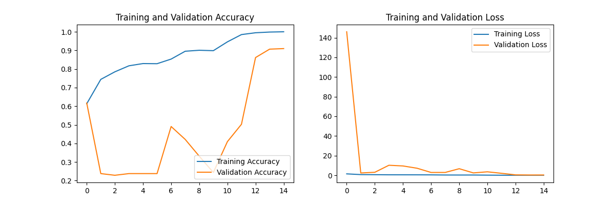

六、总结

什么是残差（Residual） ？

在深度网络中，假设某层的理想映射为 H(x)，输入为 x，则残差 F(x)=H(x)−x。残差网络通过引入短接连接（Skip Connection），将网络的学习目标从学习完整的 H(x) 转变为学习残差 F(x)。

残差的本质是目标函数的重构。它将"直接拟合目标特征"转换成了"拟合输入与目标之间的差异"。这种转换使得网络在冗余层中极易实现"恒等映射"（只需让 F(x)→0），从而彻底解决了网络加深导致的梯度消失和网络退化问题，使训练上百层甚至上千层的超深网络成为可能。

举例来说，假设你现在的成绩是 90 分（这就是输入 x）。你的终极目标是考 95 分（这就是理想输出 H(x)）。

那么，残差 F(x) 就是你需要额外努力补足的那 5 分（即 95−90=5）。

在传统的 CNN（比如 VGG-16）里，每一层都在试图直接学会怎么考出 95 分（直接学习完整的 H(x)）。

但是在 ResNet 里，网络学会了"偷懒"，它说："既然你已经有 90 分的底子了，我就只学怎么再加 5 分就好了。"

所以，数学公式表达就是：理想输出 = 残差 + 输入

即：H(x)=F(x)+x

让一个学霸从 90 分考到 95 分，只需要让他做两道压轴题（学习差值 F(x)）；但如果让他把初中高中的知识从头到尾再学一遍来保证能考 95 分（学习完整映射 H(x)），他不仅会累死，还可能学串了退步到 80 分。

神经网络也是一样，学习一个微小的"变化量"，远比从头学习一个复杂的"完整特征"要容易得多。

并且，假如网络已经足够深，前面几十层已经提取到了非常完美的特征（已经考了 100 分了），后面的层其实什么都不用做，保持原样传递下去就行。

在传统网络里，让经过了一堆 ReLU 激活函数和卷积的复杂网络去学习"什么都不做"（让输出等于输入），在数学上是极其困难的。

但在 ResNet 里，因为 H(x)=F(x)+x，如果网络发现特征已经很完美了，它只需要把残差 F(x) 的权重全部变成 0，那么 H(x) 就完美等于 x。对于神经网络来说，把一堆权重变成 0，非常简单。

模块化搭建思想：我们不再像以前那样把所有层"一锅乱炖"，而是学会了将网络封装成标准的积木模块：输入输出维度一致的 identity_block（恒等块），以及需要调整维度的 conv_block（卷积块）。利用这些基础积木，我们堆叠出了深达 50 层的 ResNet-50 完整架构，真正掌握了工业界复杂大模型的构建范式。

动态学习率 (Learning Rate Schedule)：面对千万级参数量的庞大网络，固定学习率根本行不通。所以我们编写adjust_learning_rate函数，让学习率随着 Epoch 的增加自动阶梯式减小。

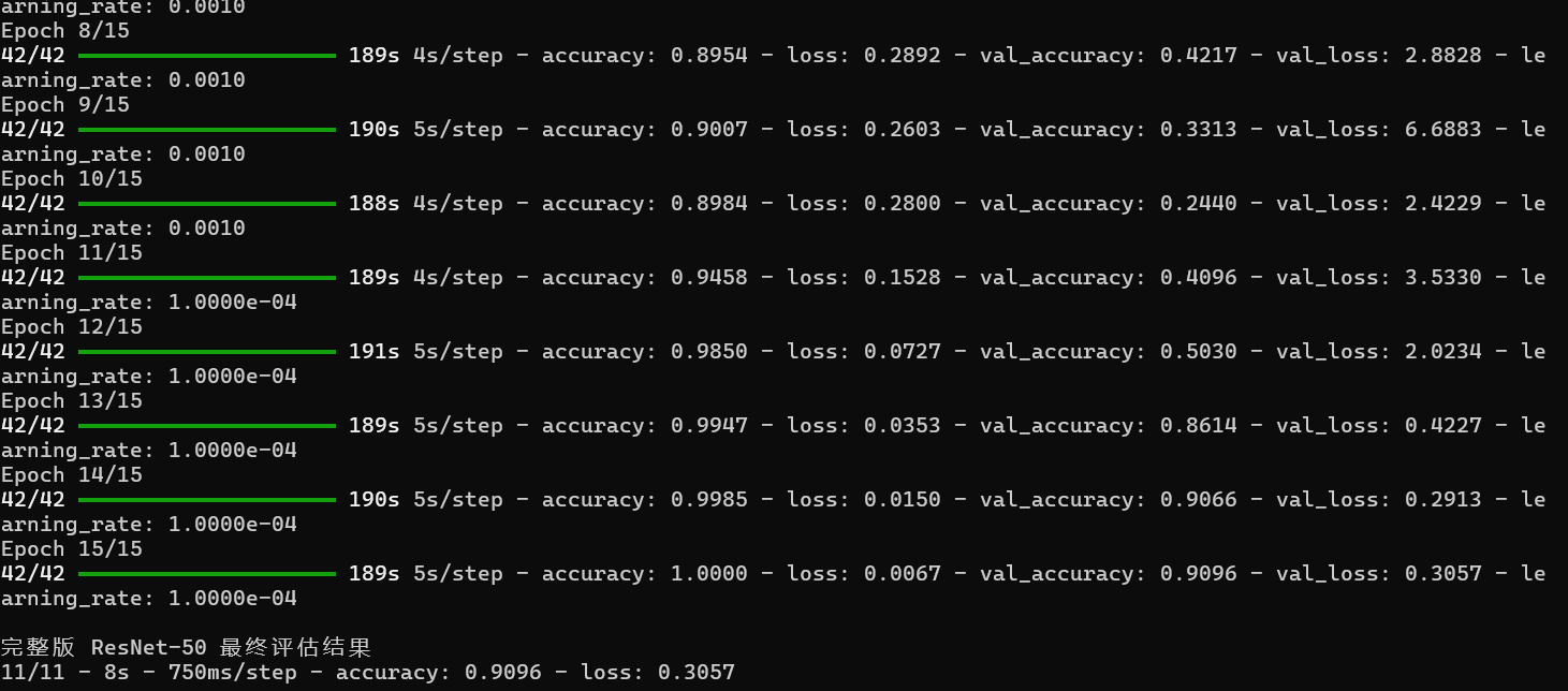
正是这种"前期大步探索，后期小步微调"的动态策略，拯救了我们在前 10 轮中 Loss 爆炸、准确率震荡的模型，最终奇迹般地拉升到了 90% 以上的高准确率。

实验结果 ：观察前 10 个 Epoch 的曲线图，出现了一个极其吓人的现象：训练集极好，验证集极差，蓝线（训练准确率）一直在稳步攀升，但橙线（验证准确率）却在 0.2 到 0.4 之间剧烈震荡，甚至一度暴跌。Loss 值从最开始的 Validation Loss 居然飙到了 140 多。

但在 Epoch 11 的时候，代码里的 lr_schedule 触发了，学习率从 0.001 骤降到了 0.0001。就在学习率下降的下一轮（Epoch 12），验证集准确率（橙线）瞬间从 0.4 狂飙到了 0.86。随后稳步上升，最终定格在极佳的 0.9096。

所以以后训练大模型，最好不要用固定学习率。前期用大学习率（0.001）让模型在巨大的参数空间里快速狂奔、寻找大致方向（即使震荡也没关系）；中后期必须调小学习率，让模型在最优解附近小心翼翼地"稳稳降落"。如果没有那一波学习率衰减，这个模型就彻底废了。

并且，"迁移学习"才是终极解法。手搭并从零训练 ResNet-50 耗时太长且极不稳定。遇到实际项目，直接加载在 ImageNet 上预训练好的权重（Transfer Learning），站在巨人的肩膀上微调，既省算力又稳定。