Chapter 002. 线性回归

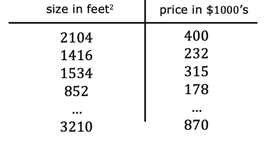
这个数据集可以帮助你估算客户可以卖多少钱

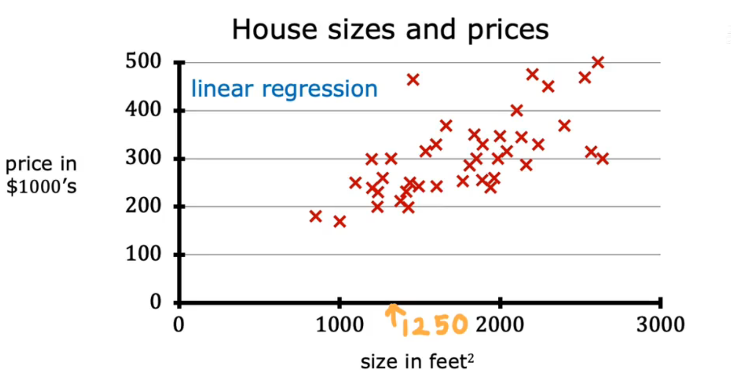
房子尺寸为1250平方英尺

从这个数据集中建立一个线性回归模型

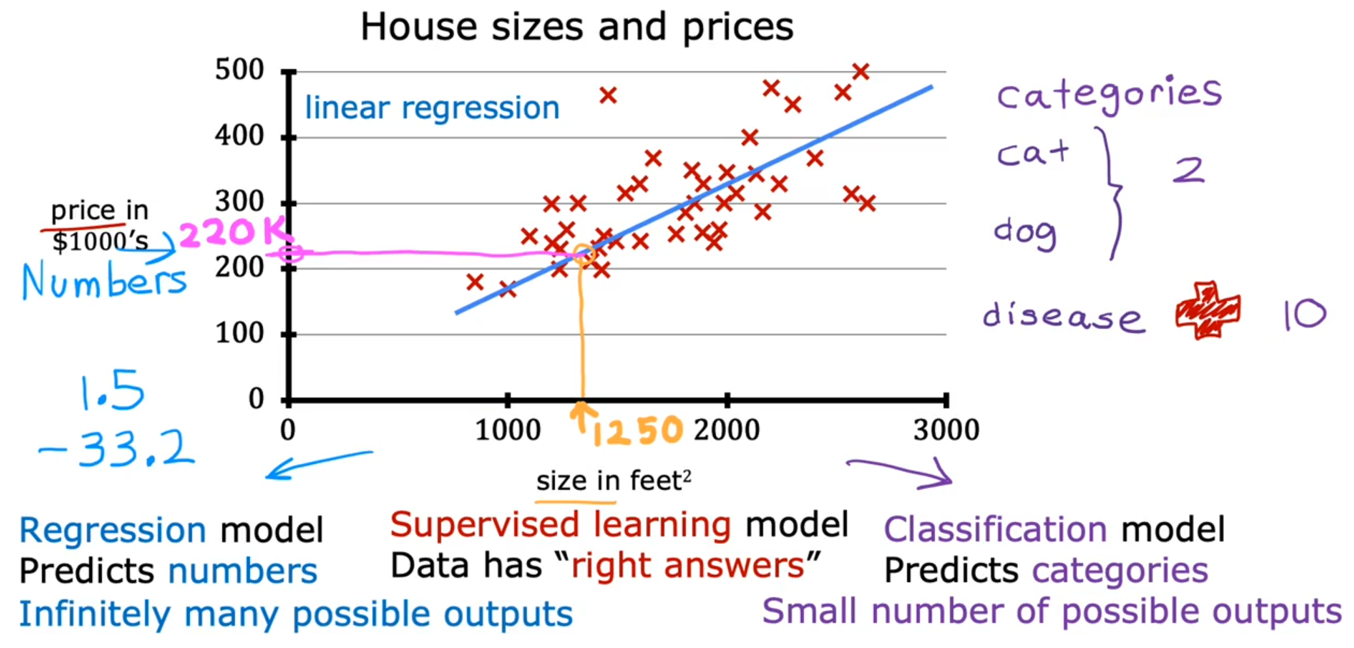
Data has "Right Answers"
Regression model -> Predicts numbers

• 问题场景：用房屋面积（单位：平方英尺）预测房价（单位：千美元）

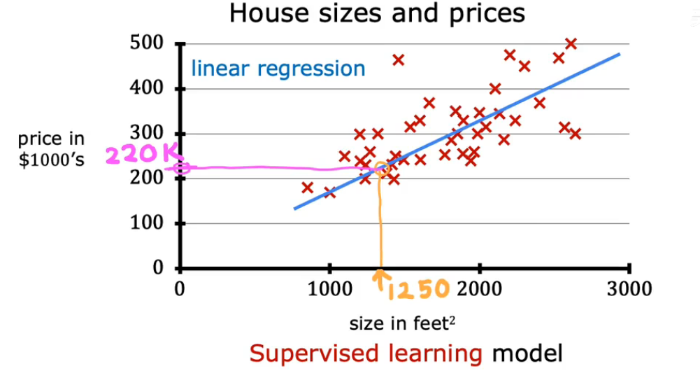
• 模型输出：连续的数值结果（如面积 1250 平方英尺时，预测房价约为 220K 美元）

• 关键特点：

  • 预测目标是数值（Numbers）
  • 存在无限多可能的输出值
  • 模型通过拟合趋势线（线性回归），建立输入特征与连续输出的映射关系
    监督学习的共性

回归与分类都属于监督学习，其核心定义为：

数据中自带 "正确答案"（标签），模型通过学习输入与标签的对应关系，实现预测。

分类模型

聚焦于预测离散类别的任务，图中给出两类典型场景：

• 二分类示例：区分 "猫" 和 "狗"，仅存在 2 种可能的输出结果

• 多分类示例：疾病诊断，可输出 10 种不同的疾病类别

• 关键特点：

  • 预测目标是类别 / 标签（Categories）
  • 输出为有限个固定的离散值

对比维度	回归模型	分类模型
预测目标	连续数值（如房价、销量、温度）	离散类别（如物种、疾病类型、用户等级）
输出空间	无限多可能的结果	有限个固定的结果
典型场景	房价预测、销量预测、股票价格预测	图像识别、垃圾邮件过滤、疾病诊断

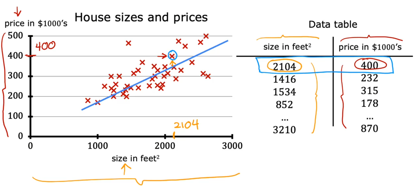
数据表格和可视化散点图

---

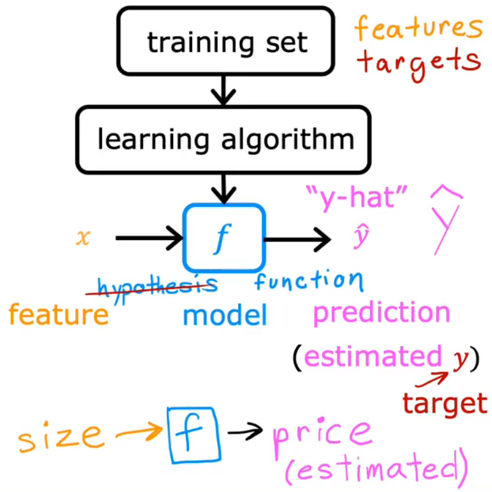
术语表

• Training set(训练集) :Data used to the model
  

• Notation

  • x = "input" variable & feature
  • y = "output" variable & "target" variable
  • m = number of training examples
  • (x , y) = single training example
  • (x(i)x^{(i)}x(i) , y(i)y^{(i)}y(i)) = i(th)i^{(th)}i(th) training example

---

Process Of How Supervised Learning Works

fw,b(x(i))=wx(i)+bf_{w,b}(x^{(i)}) = wx^{(i)}+bfw,b(x(i))=wx(i)+b

这个公式就是一条直线方程，它的作用是：

• 用 w 控制直线的斜率（面积对房价的影响程度）
• 用 b 控制直线的上下平移（调整整体预测的基准）
• 最终目标是找到合适的 w 和 b，让这条直线尽可能贴近所有训练数据点，从而实现对新数据的预测。
  

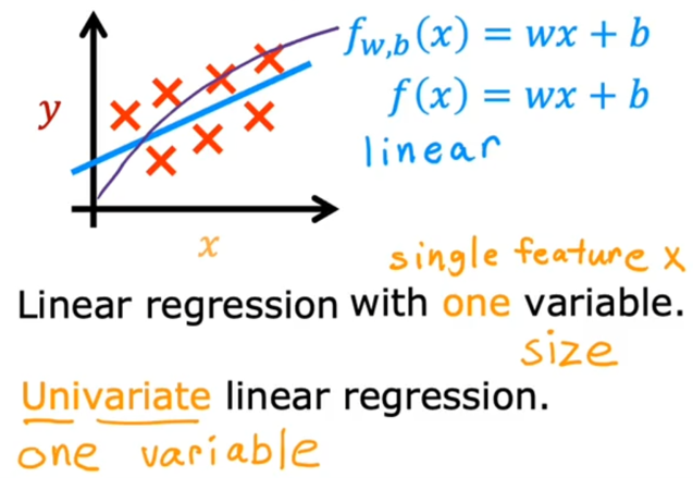
单变量线性回归（一元线性回归）

import numpy as np
import matplotlib.pyplot as plt
plt.style.use('./deeplearning.mplstyle')

# x_train is the input variable (size in 1000 square feet)
# y_train is the target (price in 1000s of dollars)
x_train = np.array([1.0, 2.0])
y_train = np.array([300.0, 500.0])
print(f"x_train = {x_train}")
print(f"y_train = {y_train}")

# m is the number of training examples
print(f"x_train.shape: {x_train.shape}")
m = x_train.shape[0]
print(f"Number of training examples is: {m}")

# m is the number of training examples
m = len(x_train)
print(f"Number of training examples is: {m}")

i = 0 # Change this to 1 to see (x^1, y^1)
x_i = x_train[i]
y_i = y_train[i]
print(f"(x^({i}), y^({i})) = ({x_i}, {y_i})")

# Plot the data points
plt.scatter(x_train, y_train, marker='x', c='r')
# Set the title
plt.title("Housing Prices")
# Set the y-axis label
plt.ylabel('Price (in 1000s of dollars)')
# Set the x-axis label
plt.xlabel('Size (1000 sqft)')
plt.show()

w = 100
b = 100
print(f"w: {w}")
print(f"b: {b}")

def compute_model_output(x, w, b):
    """
    Computes the prediction of a linear model
    Args:
      x (ndarray (m,)): Data, m examples 
      w,b (scalar)    : model parameters  
    Returns
      y (ndarray (m,)): target values
    """
    m = x.shape[0]
    f_wb = np.zeros(m)
    for i in range(m):
        f_wb[i] = w * x[i] + b
    return f_wb

tmp_f_wb = compute_model_output(x_train, w, b)

# Plot our model prediction
plt.plot(x_train, tmp_f_wb, c='b', label='Our Prediction')

# Plot the data points
plt.scatter(x_train, y_train, marker='x', c='r', label='Actual Values')

# Set the title
plt.title("Housing Prices")
# Set the y-axis label
plt.ylabel('Price (in 1000s of dollars)')
# Set the x-axis label
plt.xlabel('Size (1000 sqft)')
plt.legend()
plt.show()

# Prediction for a house with 1200 sqft
w = 200                         
b = 100    
x_i = 1.2
cost_1200sqft = w * x_i + b    

print(f"${cost_1200sqft:.0f} thousand dollars")