Fully Sparse 3D Occupancy Prediction
完全稀疏的 3D 占用预测
Haisong Liu1,2∗, Yang Chen1∗, Haiguang Wang1, Zetong Yang2, Tianyu Li2,
Jia Zeng2, Li Chen2, Hongyang Li2, Limin Wang1,2,✉
1Nanjing University 2Shanghai AI Lab
https://github.com/MCG-NJU/SparseOcc
目录
[1 Introduction](#1 Introduction)
[1 引言](#1 引言)
[2 Related Work](#2 Related Work)
[2 相关工作](#2 相关工作)
[Camera-based 3D Occupancy Prediction.](#Camera-based 3D Occupancy Prediction.)
[基于相机的 3D 占用预测。](#基于相机的 3D 占用预测。)
[Sparse Architectures for 3D Vision.](#Sparse Architectures for 3D Vision.)
[End-to-end 3D Reconstruction from Posed Images.](#End-to-end 3D Reconstruction from Posed Images.)
[Mask Transformer.](#Mask Transformer.)
[3 SparseOcc](#3 SparseOcc)
[3.1 Sparse Voxel Decoder](#3.1 Sparse Voxel Decoder)
[3.1 稀疏体素解码器](#3.1 稀疏体素解码器)
[Overall architecture.](#Overall architecture.)
[Detailed design.](#Detailed design.)
[Temporal modeling.](#Temporal modeling.)
[3.2 Mask Transformer](#3.2 Mask Transformer)
[3.2 掩码变换器](#3.2 掩码变换器)
[Mask-guided sparse sampling.](#Mask-guided sparse sampling.)
[Loss Functions.](#Loss Functions.)
[4 Ray-level mIoU](#4 Ray-level mIoU)
[4 射线级 mIoU](#4 射线级 mIoU)
[4.1 Revisiting the Voxel-level mIoU](#4.1 Revisiting the Voxel-level mIoU)
[4.1 重新审视体素级 mIoU](#4.1 重新审视体素级 mIoU)
[4.2 Mean IoU by Ray Casting](#4.2 Mean IoU by Ray Casting)
[4.2 通过光线投射计算的均值交并比](#4.2 通过光线投射计算的均值交并比)
[5 Experiments](#5 Experiments)
[5 实验](#5 实验)
[5.1 Implementation Details](#5.1 Implementation Details)
[5.1 实现细节](#5.1 实现细节)
[5.2 Main Results](#5.2 Main Results)
[5.2 主要结果](#5.2 主要结果)
[5.3 Ablations](#5.3 Ablations)
[5.3 消融研究](#5.3 消融研究)
[Sparse voxel decoder vs. dense voxel decoder.](#Sparse voxel decoder vs. dense voxel decoder.)
[稀疏体素解码器 vs. 密集体素解码器。](#稀疏体素解码器 vs. 密集体素解码器。)
[Mask Transformer.](#Mask Transformer.)
[Is a limited set of voxels sufficient to cover the scene?](#Is a limited set of voxels sufficient to cover the scene?)
[Temporal modeling.](#Temporal modeling.)
[5.4 More Studies](#5.4 More Studies)
[5.4 更多研究](#5.4 更多研究)
[The effect of training with visible masks.](#The effect of training with visible masks.)
[Panoptic occupancy.](#Panoptic occupancy.)
[5.5 Limitations](#5.5 Limitations)
[5.5 限制](#5.5 限制)
[Accumulative errors.](#Accumulative errors.)
[6 Conclusion](#6 Conclusion)
[6 结论](#6 结论)
Abstract
摘要
Occupancy prediction plays a pivotal role in autonomous driving. Previous methods typically construct dense 3D volumes, neglecting the inherent sparsity of the scene and suffering from high computational costs. To bridge the gap, we introduce a novel fully sparse occupancy network, termed SparseOcc. SparseOcc initially reconstructs a sparse 3D representation from camera-only inputs and subsequently predicts semantic/instance occupancy from the 3D sparse representation by sparse queries. A mask-guided sparse sampling is designed to enable sparse queries to interact with 2D features in a fully sparse manner, thereby circumventing costly dense features or global attention. Additionally, we design a thoughtful ray-based evaluation metric, namely RayIoU, to solve the inconsistency penalty along the depth axis raised in traditional voxel-level mIoU criteria. SparseOcc demonstrates its effectiveness by achieving a RayIoU of 34.0, while maintaining a real-time inference speed of 17.3 FPS, with 7 history frames inputs. By incorporating more preceding frames to 15, SparseOcc continuously improves its performance to 35.1 RayIoU without bells and whistles.
占用率预测在自动驾驶中起着关键作用。以往的方法通常构建密集的 3D 体素,忽略了场景固有的稀疏性,并遭受高计算成本的困扰。为了弥合这一差距,我们引入了一种新颖的全稀疏占用网络,称为 SparseOcc。SparseOcc 首先从仅基于相机的输入重建稀疏的 3D 表示,然后通过稀疏查询从 3D 稀疏表示中预测语义/实例占用。设计了一种基于掩码的稀疏采样,以使稀疏查询能够以完全稀疏的方式与 2D 特征交互,从而避免了昂贵的密集特征或全局注意力。此外,我们设计了一种深思熟虑的基于射线的评估指标,即 RayIoU,以解决传统体素级 mIoU 标准中沿深度轴的不一致惩罚。SparseOcc 通过实现 34.0 的 RayIoU,同时保持 17.3 FPS 的实时推理速度(使用 7 个历史帧输入),证明了其有效性。通过纳入更多的前置帧(达到 15 个),SparseOcc 持续改进其性能,达到 35.1 的 RayIoU,而无需额外的技巧。
1 Introduction
1 引言
Vision-centric 3D occupancy prediction [1](https://arxiv.org/html/2312.17118v5#bib.bib1 "1") focuses on partitioning 3D scenes into structured grids from visual images. Each grid is assigned a label indicating if it is occupied or not. This task offers more geometric details than 3D object detection and produces an alternative representation to LiDAR-based perception [63](https://arxiv.org/html/2312.17118v5#bib.bib63 "63"), [23](https://arxiv.org/html/2312.17118v5#bib.bib23 "23"), [60](https://arxiv.org/html/2312.17118v5#bib.bib60 "60"), [61](https://arxiv.org/html/2312.17118v5#bib.bib61 "61"), [62](https://arxiv.org/html/2312.17118v5#bib.bib62 "62"), [31](https://arxiv.org/html/2312.17118v5#bib.bib31 "31"), [32](https://arxiv.org/html/2312.17118v5#bib.bib32 "32").
以视觉为中心的 3D 占用预测1侧重于将 3D 场景从视觉图像分割成结构化网格。每个网格都被分配一个标签,指示其是否被占用。这项任务比 3D 目标检测提供了更多的几何细节,并提供了一种基于 LiDAR 感知的替代表示63, 23, 60, 61, 62, 31, 32。
(a)
(b)
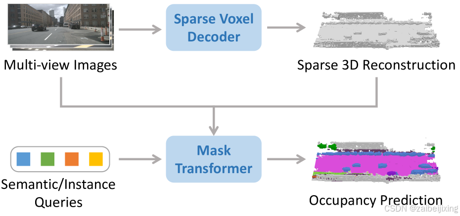
Figure 1: (a) SparseOcc reconstructs a sparse 3D representation from camera-only inputs by a sparse voxel decoder, and then estimates the mask and label of each segment via a set of sparse queries. (b) Performance comparison on the validation split of Occ3D-nuScenes. FPS is measured on a Tesla A100 with the PyTorch fp32 backend.
图 1:(a)SparseOcc 通过稀疏体素解码器从仅包含摄像头的输入中重建稀疏的 3D 表示,然后通过一组稀疏查询估计每个部分的掩码和标签。(b)在 Occ3D-nuScenes 的验证分割上的性能比较。FPS 是在带有 PyTorch fp32 后端的 Tesla A100 上测量的。
Existing methods [27](https://arxiv.org/html/2312.17118v5#bib.bib27 "27"), [16](https://arxiv.org/html/2312.17118v5#bib.bib16 "16"), [57](https://arxiv.org/html/2312.17118v5#bib.bib57 "57"), [45](https://arxiv.org/html/2312.17118v5#bib.bib45 "45"), [28](https://arxiv.org/html/2312.17118v5#bib.bib28 "28") typically construct dense 3D features yet suffer from computational overhead (e.g ., 2∼3 FPS on the Tesla A100 GPU). However, dense representations are not necessary for occupancy prediction. We statistic the geometry sparsity and find that more than 90% of the voxels are empty. This manifests a large room in occupancy prediction acceleration by exploiting the sparsity. Some works [26](https://arxiv.org/html/2312.17118v5#bib.bib26 "26"), [19](https://arxiv.org/html/2312.17118v5#bib.bib19 "19") explore the sparsity of 3D scenes, but they still rely on sparse-to-dense modules for dense predictions. This inspires us to seek a pure sparse occupancy network without any dense design.
现有方法27, 16, 57, 45, 28通常构建密集的 3D 特征,但计算开销较大(例如,在 Tesla A100 GPU 上为 2∼3 FPS)。然而,密集表示对于占用预测并不是必要的。我们统计了几何稀疏性,发现超过 90%的体素是空的。这表明通过利用稀疏性,可以大大加速占用预测。一些工作26, 19探索了 3D 场景的稀疏性,但它们仍然依赖于稀疏到密集的模块来进行密集预测。这启发我们寻求一种完全稀疏的占用网络,没有任何密集设计。
In this paper, we propose SparseOcc, the first fully sparse occupancy network. As depicted in Fig. 1 (a), SparseOcc includes two steps. First, it leverages a sparse voxel decoder to reconstruct the sparse geometry of a scene in a coarse-to-fine manner. This only models non-free regions, saving computational costs significantly. Second, we design a mask transformer with sparse semantic/instance queries to predict masks and labels of segments from the sparse space. The mask transformer not only improves performance on semantic occupancy but also paves the way for panoptic occupancy. A mask-guided sparse sampling is designed to achieve sparse cross-attention in the mask transformer. As such, our SparseOcc fully exploits the sparse property and gets rid of any dense design like dense 3D features, sparse-to-dense modules, and global attention.
本文提出了SparseOcc,这是第一个完全稀疏的占用网络。如图1(a)所示,SparseOcc包括两个步骤。首先,它利用稀疏体素解码器以粗到细的方式重建场景的稀疏几何结构。这仅建模非空区域,大大节省了计算成本。其次,我们设计了一个带有稀疏语义/实例查询的掩码变换器,用于从稀疏空间预测掩码和分割的标签。掩码变换器不仅提高了语义占用的性能,还为全景占用铺平了道路。设计了一个基于掩码的稀疏采样,以实现掩码变换器中的稀疏交叉注意力。因此,我们的 SparseOcc 充分利用了稀疏特性,摆脱了任何密集设计,如密集的 3D 特征、从稀疏到密集的模块和全局注意力。
Besides, we notice flaws in popular voxel-level mean Intersection-over-Union (mIoU) metrics for occupancy evaluation and further design a ray-level evaluation, RayIoU, as the solution. The mIoU criterion is an ill-posed formulation given the ambiguous labeling of unscanned voxels. Previous methods[50](https://arxiv.org/html/2312.17118v5#bib.bib50 "50") relieve this issue by only evaluating observed areas but raise extra issues in inconsistency penalty along depths. Instead, RayIoU addresses the two aforementioned issues simultaneously. It evaluates predicted 3D occupancy volume by retrieving depth and category predictions of designated rays. To be specific, RayIoU casts query rays into predicted 3D volumes and decides true positive predictions as the ray with the correct distance and class of its first touched occupied voxel grid. This formulates a more fair and reasonable criterion.
此外,我们注意到流行的体素级平均交并比(mIoU)指标在占用评估方面存在缺陷,并进一步设计了一种基于射线的评估方法,即 RayIoU,作为解决方案。由于未扫描体素的模糊标注,mIoU 标准是一个不适定的问题。先前的方法50通过仅评估观测区域来缓解这一问题,但在深度一致性惩罚方面引发了额外的问题。相反,RayIoU 同时解决了这两个问题。它通过检索指定射线的深度和类别预测来评估预测的 3D 占用体积。具体而言,RayIoU 将查询射线投射到预测的3D体积中,并将具有正确距离和第一个接触到的占用体素网格类别的射线判定为真阳性预测。这形成了一个更公平和合理的标准。
Thanks to the sparsity design, SparseOcc achieves 34.0 RayIoU on Occ3D-nuScenes [50](https://arxiv.org/html/2312.17118v5#bib.bib50 "50"), while maintaining a real-time inference speed of 17.3 FPS (Tesla A100, PyTorch fp32 backend), with 7 history frames inputs. By incorporating more preceding frames to 15, SparseOcc continuously improves its performance to 35.1 RayIoU, achieving state-of-the-art performance without bells and whistles. The comparison between SparseOcc with previous methods in terms of performance and efficiency is shown in Fig. 1 (b).
得益于稀疏设计,SparseOcc 在 Occ3D-nuScenes 50上实现了 34.0 RayIoU,同时保持了 17.3 FPS 的实时推理速度(Tesla A100,PyTorch fp32 后端),使用 7 个历史帧输入。通过纳入更多前置帧到 15 个,SparseOcc 持续提升其性能到 35.1 RayIoU,在不使用复杂技巧的情况下达到最先进的性能。SparseOcc 与之前方法在性能和效率方面的比较如图 1(b)所示。
We summarize our contributions as follows:
我们将我们的贡献总结如下:
-
We propose SparseOcc, the first fully sparse occupancy network without any time-consuming dense designs. It achieves 34.0 RayIoU on Occ3D-nuScenes benchmark with an real-time inference speed of 17.3 FPS.
- 我们提出了 SparseOcc,这是第一个完全稀疏的占用网络,没有任何耗时的密集设计。它在 Occ3D-nuScenes 基准测试上实现了 34.0 RayIoU,推理速度为 17.3 FPS。
-
We present RayIoU, a ray-wise criterion for occupancy evaluation. By querying rays to 3D volume, it solves the ambiguous penalty issue for unscanned free voxels and the inconsistent depth penalty issue in the mIoU metric.
2. 我们提出了 RayIoU,这是一种用于占用评估的逐射线标准。通过查询 3D 体积中的射线,它解决了未扫描的自由体素的模糊惩罚问题以及 mIoU 度量中的不一致深度惩罚问题。
2 Related Work
2 相关工作
Camera-based 3D Occupancy Prediction.
基于相机的 3D 占用预测。
The occupancy network is originally proposed by Mescheder et al . [37](https://arxiv.org/html/2312.17118v5#bib.bib37 "37"), [42](https://arxiv.org/html/2312.17118v5#bib.bib42 "42"), focusing on continuous object representations in 3D space. Recent variations [1](https://arxiv.org/html/2312.17118v5#bib.bib1 "1"), [4](https://arxiv.org/html/2312.17118v5#bib.bib4 "4"), [45](https://arxiv.org/html/2312.17118v5#bib.bib45 "45"), [50](https://arxiv.org/html/2312.17118v5#bib.bib50 "50"), [54](https://arxiv.org/html/2312.17118v5#bib.bib54 "54"), [56](https://arxiv.org/html/2312.17118v5#bib.bib56 "56"), [11](https://arxiv.org/html/2312.17118v5#bib.bib11 "11"), [58](https://arxiv.org/html/2312.17118v5#bib.bib58 "58") mostly draw inspiration from Bird's Eye View (BEV) perception [25](https://arxiv.org/html/2312.17118v5#bib.bib25 "25"), [24](https://arxiv.org/html/2312.17118v5#bib.bib24 "24"), [27](https://arxiv.org/html/2312.17118v5#bib.bib27 "27"), [16](https://arxiv.org/html/2312.17118v5#bib.bib16 "16"), [15](https://arxiv.org/html/2312.17118v5#bib.bib15 "15"), [18](https://arxiv.org/html/2312.17118v5#bib.bib18 "18"), [17](https://arxiv.org/html/2312.17118v5#bib.bib17 "17"), [55](https://arxiv.org/html/2312.17118v5#bib.bib55 "55"), [34](https://arxiv.org/html/2312.17118v5#bib.bib34 "34"), [35](https://arxiv.org/html/2312.17118v5#bib.bib35 "35"), [30](https://arxiv.org/html/2312.17118v5#bib.bib30 "30"), [33](https://arxiv.org/html/2312.17118v5#bib.bib33 "33"), [53](https://arxiv.org/html/2312.17118v5#bib.bib53 "53"), [59](https://arxiv.org/html/2312.17118v5#bib.bib59 "59") and predicts voxel-level semantic information from image inputs. For instance, MonoScene[4](https://arxiv.org/html/2312.17118v5#bib.bib4 "4") estimates occupancy through a 2D and a 3D UNet [43](https://arxiv.org/html/2312.17118v5#bib.bib43 "43") connected by a sight projection module. SurroundOcc[57](https://arxiv.org/html/2312.17118v5#bib.bib57 "57") proposes a coarse-to-fine architecture. However, the large number of voxel queries is computationally heavy. TPVFormer[19](https://arxiv.org/html/2312.17118v5#bib.bib19 "19") proposes tri-perspective view representations to supplement vertical structural information, but this inevitably leads to information loss. VoxFormer[26](https://arxiv.org/html/2312.17118v5#bib.bib26 "26") initializes sparse queries based on monocular depth prediction. Nevertheless, VoxFormer is not fully sparse as it still requires a sparse-to-dense MAE[13](https://arxiv.org/html/2312.17118v5#bib.bib13 "13") module to complete the scene. Some methods emerged in the CVPR 2023 occupancy challenge[28](https://arxiv.org/html/2312.17118v5#bib.bib28 "28"), [40](https://arxiv.org/html/2312.17118v5#bib.bib40 "40"), [9](https://arxiv.org/html/2312.17118v5#bib.bib9 "9"), but none of them exploits a fully sparse design. In this paper, we make the first step to explore the fully sparse architecture for 3D occupancy prediction from camera-only inputs.
占用网络最初由 Mescheder 等人37, 42提出,重点关注 3D 空间中的连续物体表示。最近的变体1, 4, 45, 50, 54, 56, 11, 58大多从鸟瞰图(BEV)感知25, 24, 27, 16, 15, 18, 17, 55, 34, 35, 30, 33, 53, 59中汲取灵感,并从图像输入中预测体素级别的语义信息。例如,MonoScene4通过一个由视线投影模块连接的 2D 和 3D UNet43来估计占用情况。SurroundOcc57提出了一种从粗到细的架构。然而,大量的体素查询在计算上很繁重。TPVFormer19提出了三视角视图表示来补充垂直结构信息,但这不可避免地会导致信息丢失。VoxFormer26基于单目深度预测初始化稀疏查询。然而,VoxFormer 并不完全稀疏,因为它仍然需要一个稀疏到密集的 MAE 13模块来完成场景。一些方法在 CVPR 2023 占用挑战28, 40, 9中出现,但没有一个利用完全稀疏的设计。在本文中,我们迈出了探索仅基于摄像头输入的 3D 占用预测完全稀疏架构的第一步。
Sparse Architectures for 3D Vision.
三维视觉的稀疏架构。
Sparse architectures find widespread adoption in LiDAR-based reconstruction [48](https://arxiv.org/html/2312.17118v5#bib.bib48 "48") and perception [7](https://arxiv.org/html/2312.17118v5#bib.bib7 "7"), [63](https://arxiv.org/html/2312.17118v5#bib.bib63 "63"), [60](https://arxiv.org/html/2312.17118v5#bib.bib60 "60"), [61](https://arxiv.org/html/2312.17118v5#bib.bib61 "61"), leveraging the inherent sparsity of point clouds. However, when it comes to vision-to-3D tasks, a direct adaptation is not feasible due to the absence of point cloud inputs. A prior work, SparseBEV [33](https://arxiv.org/html/2312.17118v5#bib.bib33 "33"), proposes a fully sparse architecture for camera-based 3D object detection. Nevertheless, directly adapting this approach is non-trivial because 3D object detection focuses on a sparse set of objects, whereas 3D occupancy requires dense predictions for each voxel. Consequently, designing a fully sparse architecture for 3D occupancy prediction remains a challenging task.
稀疏架构在基于 LiDAR 的重建48和感知7, 63, 60, 61中得到了广泛应用,利用了点云固有的稀疏性。然而,在视觉到 3D 的任务中,直接适应是不可能的,因为缺乏点云输入。之前的一项工作 SparseBEV33提出了一种完全稀疏的架构用于基于相机的 3D 目标检测。然而,直接采用这种方法并不简单,因为 3D 目标检测关注的是一组稀疏的目标,而 3D 占有率需要对每个体素进行密集预测。因此,设计一个用于 3D 占有率预测的完全稀疏架构仍然是一个具有挑战性的任务。
End-to-end 3D Reconstruction from Posed Images.
从姿态图像进行端到端的三维重建。
As a related task to 3D occupancy prediction, 3D reconstruction recovers the 3D geometry from multiple posed images. Recent methods focus on more compact and efficient end-to-end 3D reconstruction pipelines [39](https://arxiv.org/html/2312.17118v5#bib.bib39 "39"), [47](https://arxiv.org/html/2312.17118v5#bib.bib47 "47"), [2](https://arxiv.org/html/2312.17118v5#bib.bib2 "2"), [46](https://arxiv.org/html/2312.17118v5#bib.bib46 "46"), [10](https://arxiv.org/html/2312.17118v5#bib.bib10 "10"). Atlas [39](https://arxiv.org/html/2312.17118v5#bib.bib39 "39") extracts features from multi-view input images and maps them to 3D space to construct the truncated signed distance function [8](https://arxiv.org/html/2312.17118v5#bib.bib8 "8"). NeuralRecon [47](https://arxiv.org/html/2312.17118v5#bib.bib47 "47") directly reconstructs local surfaces as sparse TSDF volumes and uses a GRU-based TSDF fusion module to fuse features from previous fragments. VoRTX [46](https://arxiv.org/html/2312.17118v5#bib.bib46 "46") utilizes transformers to address occlusion issues in multi-view images.
作为 3D 占用预测的关联任务,3D 重建从多视角图像中恢复 3D 几何形状。近期的方法重点关注更紧凑和高效的端到端 3D 重建流水线39, 47, 2, 46, 10。Atlas39从多视角输入图像中提取特征并将其映射到 3D 空间,以构建截断符号距离函数8。NeuralRecon47直接重建局部表面作为稀疏的 TSDF 体素,并使用基于 GRU 的 TSDF 融合模块融合之前片段的特征。VoRTX46利用 Transformer 解决多视角图像中的遮挡问题。
Mask Transformer.
掩码变换器。
Recently, unified segmentation models have been widely studied to handle semantic and instance segmentation concurrently. Cheng et al . first propose MaskFormer [6](https://arxiv.org/html/2312.17118v5#bib.bib6 "6") for unified segmentation in terms of model architecture, loss functions, and training strategies. Mask2Former [5](https://arxiv.org/html/2312.17118v5#bib.bib5 "5") then introduces masked attention, with restricted receptive fields on instance masks, for better performance. Later on, Mask3D [44](https://arxiv.org/html/2312.17118v5#bib.bib44 "44") successfully extends the mask transformer for point cloud segmentation with state-of-the-art performance. OpenMask3D [49](https://arxiv.org/html/2312.17118v5#bib.bib49 "49") further achieves the open-vocabulary 3D instance segmentation task and proposes a model for zero-shot 3D segmentation.
近期,统一分割模型被广泛研究以同时处理语义和实例分割。Cheng 等人首次提出了 MaskFormer 6,在模型架构、损失函数和训练策略方面统一了分割。随后,Mask2Former 5引入了掩码注意力,对实例掩码进行了受限的感受野,从而提高了性能。后来,Mask3D 44成功将掩码变换器扩展到点云分割,并取得了最先进的性能。OpenMask3D 49进一步实现了开放词汇的 3D 实例分割任务,并提出了一个用于零样本 3D 分割的模型。
3 SparseOcc
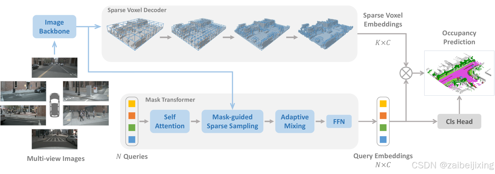
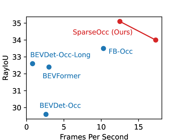
Figure 2: SparseOcc is a fully sparse architecture since it neither relies on dense 3D feature, nor has sparse-to-dense and global attention operations. The sparse voxel decoder reconstructs the sparse geometry of the scene, consisting of K voxels (K≪W×H×D). The mask transformer then uses N sparse queries to predict the mask and label of each segment. SparseOcc can be easily extended to panoptic occupancy by replacing the semantic queries with instance queries.
图 2:SparseOcc 是一种完全稀疏的架构,因为它既不依赖于密集的 3D 特征,也没有稀疏到密集和全局注意力操作。稀疏体素解码器重建了场景的稀疏几何结构,由 K 个体素(K≪W×H×D)组成。然后,掩码变换器使用 N 稀疏查询来预测每个部分的掩码和标签。SparseOcc 可以通过用实例查询替换语义查询来轻松扩展到全景占用。
SparseOcc is a vision-centric occupancy model that only requires camera inputs. As shown in Fig. 2, SparseOcc has three modules: an image encoder consisting of an image backbone and FPN [29](https://arxiv.org/html/2312.17118v5#bib.bib29 "29") to extract 2D features from multi-view images; a sparse voxel decoder (Sec. 3.1) to predict sparse class-agnostic 3D occupancy with correlated embeddings from the image features; a mask transformer decoder (Sec 3.2) to distinguish semantics and instances in the sparse 3D space.
SparseOcc 是一个以视觉为中心的占用模型,仅需相机输入。如图 2 所示,SparseOcc 有三个模块:一个由图像主干和 FPN 29组成的图像编码器,用于从多视角图像中提取 2D 特征;一个稀疏体素解码器(第 3.1 节),用于预测来自图像特征的关联嵌入的稀疏类别无关 3D 占用;一个掩码变换器解码器(第 3.2 节),用于区分稀疏 3D 空间中的语义和实例。
3.1 Sparse Voxel Decoder
3.1 稀疏体素解码器
Since 3D occupancy ground truth [50](https://arxiv.org/html/2312.17118v5#bib.bib50 "50"), [45](https://arxiv.org/html/2312.17118v5#bib.bib45 "45"), [57](https://arxiv.org/html/2312.17118v5#bib.bib57 "57"), [54](https://arxiv.org/html/2312.17118v5#bib.bib54 "54") is a dense volume with dimensions W×H×D (e.g ., 200×200×16), existing methods typically build a dense 3D feature of shape W×H×D×C, but suffer from computational overhead. In this paper, we argue that such dense representation is not necessary for occupancy prediction. As in our statistics, we find that over 90% of the voxels in the scene are free. This motivates us to explore a sparse 3D representation that only models the non-free areas of the scene, thereby saving computational resources.
由于 3D 占用地面真值50, 45, 57, 54是一个具有 W×H×D 维度(例如,200 × 200 × 16)的密集体,现有方法通常构建一个形状为 W×H×D×C 的密集 3D 特征,但会带来计算开销。在本文中,我们认为这种密集表示对于占用预测是不必要的。根据我们的统计,我们发现场景中超过 90%的体素是空闲的。这促使我们探索一种稀疏的 3D 表示,只对场景的非空闲区域进行建模,从而节省计算资源。
Overall architecture.
总体架构。
Our designed sparse voxel decoder is shown in Fig. 3. In general, it follows a coarse-to-fine structure but only models the non-free regions. The decoder starts from a set of coarse voxel queries equally distributed in the 3D space (e.g ., 25×25). In each layer, we first upsample each voxel by 2×, e.g ., a voxel with size d will be upsampled into 8 voxels with size d/2. Next, we estimate an occupancy score for each voxel and conduct pruning to remove useless voxel grids. Here we have two approaches for pruning: one is based on a threshold (e.g ., only keeps score > 0.5); the other is by top-k selection. In our implementation, we simply keep voxels with top-k occupancy scores for training efficiency. k is a dataset-related parameter, obtained by counting the maximum number of non-free voxels in each sample at different resolutions. The voxel tokens after pruning will serve as the input for the next layer.
我们设计的稀疏体素解码器如图 3 所示。通常,它遵循从粗到细的结构,但只对非空区域进行建模。解码器从一组均匀分布在 3D 空间中的粗体素查询开始(例如,25 × 25)。在每一层,我们首先将每个体素上采样 2 × 倍,例如,一个大小为 d 的体素将被上采样为 8 个大小为 d/2 的体素。接下来,我们为每个体素估计一个占用分数并进行剪枝以去除无用的体素网格。这里我们有两种剪枝方法:一种是基于阈值(例如,只保留分数>0.5);另一种是通过top-k选择。在我们的实现中,为了训练效率,我们简单地保留具有top-k占用分数的体素。k是一个与数据集相关的参数,通过在不同分辨率下计算每个样本中最大非空体素数获得。剪枝后的体素标记将作为下一层的输入。
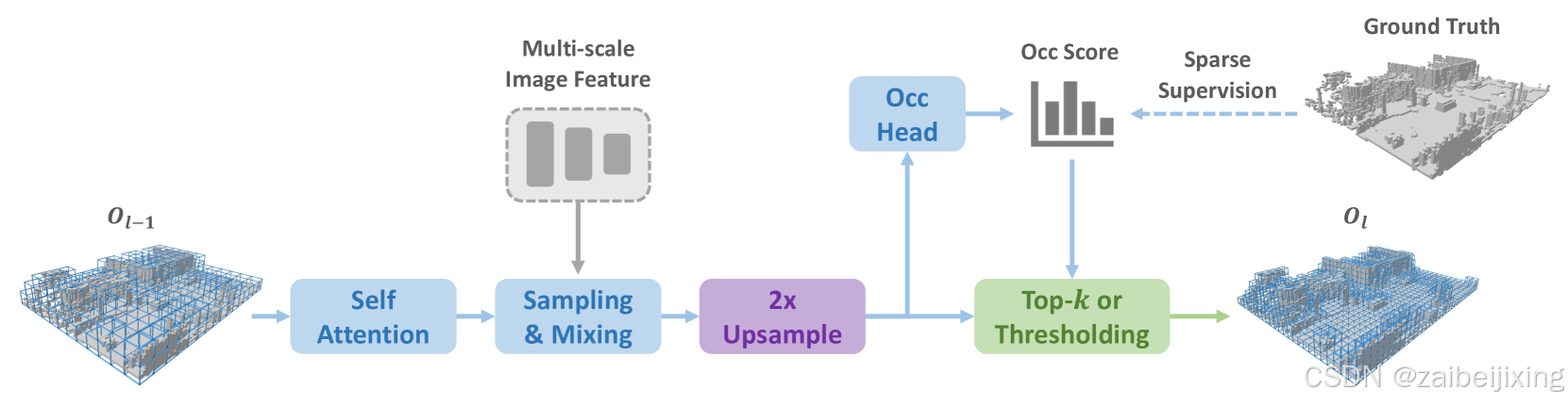
Figure 3: The sparse voxel decoder employs a coarse-to-fine pipeline with three layers. Within each layer, we utilize a transformer-like architecture for 3D-2D interaction. At the end of every layer, the voxel resolution is upsampled by a factor of 2×, and probabilities of voxel occupancy are estimated.
图 3:稀疏体素解码器采用从粗到细的流水线,包含三层。在每一层中,我们使用类似 Transformer 的架构进行 3D 到 2D 的交互。在每一层结束时,体素分辨率会以 2 倍的因子进行上采样,并估计体素占用的概率。
Detailed design.
详细设计
Within each layer, we use a transformer-like [52](https://arxiv.org/html/2312.17118v5#bib.bib52 "52") architecture to handle voxel queries. The concrete architecture is inspired by SparseBEV [33](https://arxiv.org/html/2312.17118v5#bib.bib33 "33"), a detection method using a sparse scheme. To be specific, in layer l with Kl−1 voxel queries described by 3D locations and a C-dim content vector, we first use self-attention to aggregate local and global features for those query voxels. Then, a linear layer is used to generate 3D sampling offsets {(Δxi,Δyi,Δzi)} for each voxel query from the associated content vector. These sampling offsets are utilized to transform voxel queries to obtain reference points in global coordinates. We finally project those sampled reference points to multi-view image space for integrating image features by adaptive mixing [12](https://arxiv.org/html/2312.17118v5#bib.bib12 "12"), [51](https://arxiv.org/html/2312.17118v5#bib.bib51 "51"), [20](https://arxiv.org/html/2312.17118v5#bib.bib20 "20"). In summary, our approach differs from SparseBEV by shifting the query formulation from pillars to 3D voxels. Other components such as self attention, adaptive sampling and mixing are directly borrowed.
在每一层中,我们使用类似于Transformer的52架构来处理体素查询。具体的架构受到 SparseBEV33的启发,这是一种使用稀疏方案的检测方法。具体来说,在层 l 中,有 Kl−1 个体素查询,这些查询由3D位置和 C维的内容向量描述,我们首先使用自注意力来聚合局部和全局特征,以获取这些查询体素。然后,使用一个线性层根据关联的内容向量为每个体素查询生成 3D采样偏移量 {(Δxi,Δyi,Δzi)} 。这些采样偏移量用于将体素查询转换为全局坐标中的参考点。最后,我们将这些采样的参考点投影到多视图图像空间中,通过自适应混合12, 51, 20来整合图像特征。总之,我们的方法与 SparseBEV 的不同之处在于将查询公式从柱状结构转换为 3D体素。其他组件如自注意力、自适应采样和混合则直接借鉴。
Temporal modeling.
时间建模。
Previous dense occupancy methods [27](https://arxiv.org/html/2312.17118v5#bib.bib27 "27"), [16](https://arxiv.org/html/2312.17118v5#bib.bib16 "16") typically warp the history BEV/3D feature to the current timestamp, and use deformable attention [64](https://arxiv.org/html/2312.17118v5#bib.bib64 "64") or 3D convolutions to fuse temporal information. However, this approach is not directly applicable in our case due to the sparse nature of our 3D features. To handle this, we leverage the flexibility of the aforementioned global sampled reference points by warping them to previous timestamps to sample history multi-view image features. The sampled multi-frame features are stacked and aggregated by adaptive mixing so as for temporal modeling.
先前的密集占用方法27, 16通常将历史 BEV/3D 特征扭曲到当前时间戳,并使用可变形注意力64或 3D 卷积融合时间信息。然而,由于我们 3D 特征的稀疏性,这种方法不直接适用于我们的场景。为了解决这个问题,我们利用之前提到的全局采样参考点,将它们扭曲到之前的时戳以采样历史多视角图像特征。采样的多帧特征通过自适应混合进行堆叠和聚合,以实现时间建模。
Supervision.
监督。
We compute loss for the sparsified voxels from each layer. We use binary cross entropy (BCE) loss as the supervision, given that we are reconstructing a class-agnostic sparse occupancy space. Only the kept sparse voxels are supervised, while the discarded regions during pruning in earlier stages are ignored.
我们为每个层的稀疏体素计算损失。我们使用二元交叉熵(BCE)损失作为监督,因为我们正在重建一个与类别无关的稀疏占据空间。只有保留的稀疏体素受到监督,而早期阶段修剪时丢弃的区域被忽略。
Moreover, due to the severe class imbalance, the model can be easily dominated by categories with a large proportion, such as the ground, thereby ignoring other important elements in the scene, such as cars, people, etc. Therefore, voxels belonging to different classes are assigned with different loss weights. For example, voxels belonging to class c are assigned with a loss weight of:
此外,由于严重的类别不平衡,模型很容易被具有较大比例的类别所主导,例如地面,从而忽略了场景中的其他重要元素,如汽车、人等。因此,属于不同类别的体素被分配了不同的损失权重。例如,属于类别 c 的体素被分配的损失权重为:
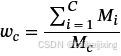
where Mi is the number of voxels belonging to the i-th class in ground truth.
其中 Mi 是属于 i 类的体素数量。
3.2 Mask Transformer
3.2 掩码变换器
Our mask transformer is inspired by Mask2Former [5](https://arxiv.org/html/2312.17118v5#bib.bib5 "5"), which uses N sparse semantic/instance queries decoupled by binary mask queries 𝐐m∈0,1N×K and content vectors 𝐐c∈ℝN×C. The mask transformer consists of three steps: multi-head self attention (MHSA), mask-guided sparse sampling, and adaptive mixing. MHSA is used for the interaction between different queries as the common practice. Mask-guided sparse sampling and adaptive mixing are responsible for the interaction between queries and 2D image features.
我们的掩码变换器受到 Mask2Former 5 的启发,它使用由二进制掩码查询 𝐐m∈0,1N×K 和内容向量 𝐐c∈ℝN×C 解耦的 N 稀疏语义/实例查询。掩码变换器由三个步骤组成:多头自注意力(MHSA)、掩码引导的稀疏采样和自适应混合。MHSA 用于不同查询之间的交互,这是常见的做法。掩码引导的稀疏采样和自适应混合负责查询与 2D 图像特征之间的交互。
Mask-guided sparse sampling.
掩码引导的稀疏采样。
A simple baseline of mask transformer is to use the masked cross-attention module in Mask2Former. However, it attends to all positions of the key, with unbearable computations. Here, we design a simple alternative. We first randomly select a set of 3D points within the mask predicted by the previous (l−1)-th Transformer decoder layer. Then, we project those 3D points to multi-view images and extract their features by bilinear interpolation. Besides, our sparse sampling mechanism makes the temporal modeling easier by simply warping the sampling points (as done in the sparse voxel decoder).
一个简单的掩码变换器基线是使用 Mask2Former 中的掩码交叉注意力模块。然而,它会关注所有位置的键,计算量大得难以承受。在这里,我们设计了一个简单的替代方案。我们首先随机选择一组 3D 点,这些点位于之前( l−1 )-th Transformer 解码器层预测的掩码内。然后,我们将这些 3D 点投影到多视图图像上,并通过双线性插值提取它们的特征。此外,我们的稀疏采样机制通过简单地扭曲采样点(如稀疏体素解码器中所做的那样)使时间建模更加容易。
Prediction.
预测。
For class prediction, we apply a linear classifier with a sigmoid activation based on the query embeddings 𝐐c. For mask prediction, the query embeddings are converted to mask embeddings by an MLP. The mask embeddings 𝐌∈ℝQ×C have the same shape as query embeddings 𝐐c and are dot-producted with the sparse voxel embeddings 𝐕∈ℝK×C to produce mask predictions. Thus, the prediction space of our mask transformer is constrained to the sparsified 3D space from the sparse voxel decoder, rather than the full 3D scene. The mask predictions will serve as the mask queries 𝐐m for the next transformer layer.
对于类别预测,我们基于查询嵌入 𝐐c 应用一个带有 sigmoid 激活的线性分类器。对于掩码预测,查询嵌入通过一个 MLP 转换为掩码嵌入。掩码嵌入 𝐌∈ℝQ×C 与查询嵌入 𝐐c 形状相同,并与稀疏体素嵌入 𝐕∈ℝK×C 进行点积以生成掩码预测。因此,我们的掩码变换器的预测空间被限制在从稀疏体素解码器得到的稀疏化 3D 空间中,而不是完整的 3D 场景。掩码预测将作为下一个变换器的掩码查询 𝐐m 。
Supervision.
监督。
The reconstruction result from the sparse voxel decoder may not be reliable, as it may overlook or inaccurately detect certain elements. Thus, supervising the mask transformer presents certain challenges since its predictions are confined within this unreliable space. In cases of missed detection, where some ground truth segments are absent in the predicted sparse occupancy, we opt to discard these segments to prevent confusion. As for inaccurately detected elements, we simply categorize them as an additional "no object" category.
重建结果可能不可靠,因为它可能会忽略或错误地检测某些元素。因此,监督掩码变换器会面临一些挑战,因为它的预测被限制在这个不可靠的空间内。在漏检的情况下,如果某些地面真实片段在预测的稀疏占用中缺失,我们选择丢弃这些片段以防止混淆。至于检测不准确的元素,我们简单地将它们归类为额外的"无对象"类别。
Loss Functions.
损失函数。
Following MaskFormer [6](https://arxiv.org/html/2312.17118v5#bib.bib6 "6"), we match the ground truth with the predictions using Hungarian matching. Focal loss Lfocal is used for classification, while a combination of DICE loss [38](https://arxiv.org/html/2312.17118v5#bib.bib38 "38") Ldice and BCE mask loss Lmask is used for mask prediction. Thus, the total loss of SparseOcc is composed of four parts:
在 MaskFormer 6之后,我们使用匈牙利匹配将地面实况与预测进行匹配。Focal loss Lfocal 用于分类,而 DICE loss 38 Ldice 和 BCE mask loss Lmask 的组合用于掩码预测。因此,SparseOcc 的总损失由四部分组成:
|---|----------------------------------------|---|-----|
| | L=Lfocal+Lmask+Ldice+Locc, | | (2) |
where Locc is the loss of sparse voxel decoder.
其中 Locc 是稀疏体素解码器的损失。
4 Ray-level mIoU
4 射线级 mIoU
4.1 Revisiting the Voxel-level mIoU
4.1 重新审视体素级 mIoU
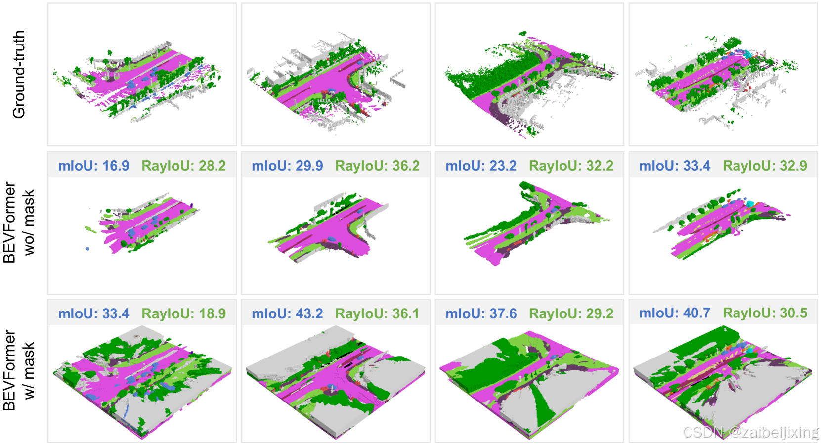
Figure 4: Visualization of the discrepancy between qualitative and quantitative results. We observe that training existing dense occupancy methods (e.g . BEVFormer) with a visible mask results in a thick surface, leading to an unreasonably inflated improvement in the current mIoU metrics. In contrast, our new RayIoU metrics provide a more accurate reflection of model performance.
图 4:定性与定量结果之间差异的可视化。我们观察到,使用可见掩码训练现有的密集占用方法(例如 BEVFormer)会导致表面变厚,从而导致当前 mIoU 指标不合理地膨胀。相比之下,我们的新 RayIoU 指标能更准确地反映模型性能。
The Occ3D dataset [50](https://arxiv.org/html/2312.17118v5#bib.bib50 "50"), along with its proposed evaluation metrics, are widely recognized as benchmarks in this field. The ground truth occupancy is reconstructed from LiDAR point clouds, and the mean Intersection over Union (mIoU) at the voxel level is employed to assess performance. Due to factors such as distance and occlusion, the accumulated point clouds are not perfect. Some areas unscanned by LiDAR are marked as free, resulting in fragmented instances. This raises the problem of label inconsistency. To solve this problem, Occ3D uses a binary visible mask that indicates whether a voxel is observed in the current camera view. Only the observed voxels contribute to evaluation.
Occ3D 数据集50及其提出的评估指标被广泛认可为该领域的基准。地面真实占用情况从 LiDAR 点云中重建,并在体素级别使用平均交并比(mIoU)来评估性能。由于距离和遮挡等因素,累积的点云并不完美。一些未被 LiDAR 扫描的区域被标记为空闲,导致实例碎片化。这引发了标签不一致的问题。为了解决这个问题,Occ3D 使用了一个二值可见性掩膜,指示体素是否在当前相机视图中可见。只有被观察到的体素对评估有贡献。
However, we found that solely calculating mIoU on the observed voxel positions remains vulnerable and can be hacked by predicting a thicker surface. Dense methods (e.g ., BEVFormer [27](https://arxiv.org/html/2312.17118v5#bib.bib27 "27")) can easily achieve this by training with the visible mask. During training, the area behind the surface lacks supervision, causing the model to fill it with duplicated predictions, resulting in a thicker surface. As an example, consider BEVFormer, which generates a thick and noisy surface when trained with the visible mask (see Fig. 4). Despite this, its performance exhibits an unreasonably inflated improvement (+5∼15 mIoU) under the current evaluation protocol.
然而,我们发现仅在观察到的体素位置上计算 mIoU 仍然存在漏洞,并且可以通过预测更厚的表面来破解。密集方法(例如,BEVFormer 27)可以通过使用可见掩码进行训练轻松实现这一点。在训练过程中,表面后面的区域缺乏监督,导致模型用重复预测填充该区域,从而产生更厚的表面。例如,考虑使用可见掩码训练的 BEVFormer,它会产生厚而嘈杂的表面(见图 4)。尽管如此,其性能在当前评估协议下显示出不合理的膨胀改进(+5 ∼ 15 mIoU)。
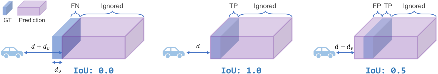
Figure 5: Illustration of inconsistent depth penalties caused by current metrics. Consider a scenario where we have a wall in front of us, with a ground-truth distance of d and a thickness of dv. When the prediction has a thickness of dp≫dv, we encounter an inconsistent penalty along depth. Specifically, if the predicted wall is dv farther than the ground truth (total distance d+dv), its IoU will be zero. Conversely, if the predicted wall is dv closer than the ground truth (total distance d−dv), the IoU remains at 0.5. This occurs because all voxels behind the surface are filled with duplicated predictions. Similarly, when the predicted depth is d−2dv, the resulting IoU is 13, and so forth.
图 5:展示了当前指标导致的不一致深度惩罚。考虑一个场景,我们面前有一堵墙,其真实距离为 d ,厚度为 dv 。当预测的厚度为 dp≫dv 时,我们会遇到沿深度方向的不一致惩罚。具体来说,如果预测的墙比真实墙远 dv (总距离为 d+dv ),其 IoU 将为零。相反,如果预测的墙比真实墙近 dv (总距离为 d−dv ),IoU 仍为 0.5。这是因为表面后面的所有体素都填充了重复的预测。类似地,当预测深度为 d−2dv 时,IoU 为 13 ,以此类推。
The misalignment between qualitative and quantitative results is caused by the inconsistent penalty along the depth direction. A toy example in Fig. 5 reveals several issues with the current metrics:
深度方向上惩罚的不一致导致了定性和定量结果之间的错位。图 5 中的玩具示例揭示了当前指标存在的几个问题:
- If the model fills all areas behind the surface, it inconsistently penalizes depth predictions. The model can obtain a higher IoU by filling all areas behind the surface and predicting a closer depth. This thick surface issue is very common in dense models trained with visible masks or 2D supervision.
- 如果模型填充了表面后的所有区域,它会不一致地惩罚深度预测。模型可以通过填充表面后的所有区域并预测更接近的深度来获得更高的 IoU。这种厚表面的问题在使用可见掩膜或 2D 监督训练的密集模型中非常常见。
- If the predicted occupancy represents a thin surface, the penalty becomes overly strict. Even a deviation of just one voxel results in an IoU of zero.
2. 如果预测的占有率表示一个薄表面,惩罚就会变得过于严格。即使是单个体素的偏差也会导致 IoU 为零。 - The visible mask only considers the visible area at the current moment, reducing occupancy prediction to a depth estimation task and overlooking the scene completion ability.
3. 可见掩膜仅考虑当前时刻的可见区域,将占有率预测减少为深度估计任务,而忽视了场景补全能力。
4.2 Mean IoU by Ray Casting
4.2 通过光线投射计算的均值交并比
To address the above issues, we propose a new evaluation metric: Ray-level mIoU (RayIoU for short). In RayIoU, the set elements are query rays rather than voxels. We emulate LiDAR behavior by projecting query rays into the predicted 3D occupancy volume. For each query ray, we compute the distance it travels before intersecting any surface and retrieve the corresponding class label. We then apply the same procedure to the ground-truth occupancy to obtain the ground-truth depth and class label. In case a ray does not intersect with any voxel present in the ground truth, it will be excluded from the evaluation process.
为了解决上述问题,我们提出了一种新的评估指标:Ray-level mIoU(简称 RayIoU)。在 RayIoU 中,集合的元素是查询射线而不是体素。我们通过将查询射线投影到预测的 3D 占有率体中来模拟 LiDAR 的行为。对于每个查询射线,我们计算它在与任何表面相交之前行进的距离,并检索相应的类别标签。然后,我们对地面实况占有率应用相同的过程,以获得地面实况深度和类别标签。如果射线与地面实况中存在的任何体素都不相交,则该射线将从评估过程中排除。
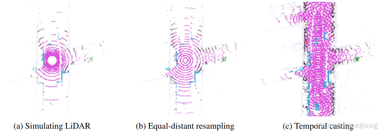
Figure 6: Covered area of RayIoU. (a) The raw LiDAR ray samples are unbalanced at different distances. (b) We resample the rays to balance the weight on distance. (c) To investigate the performance of scene completion, we propose evaluating occupancy in the visible area on a wide time span, by casting rays on visited waypoints.
图 6:RayIoU 覆盖区域。(a)原始 LiDAR 射线样本在不同距离上分布不均衡。(b)我们对射线进行重采样以平衡距离上的权重。(c)为了研究场景补全的性能,我们提出通过在已访问的航点上投射射线,在广泛的时间跨度内评估可见区域内的占有率。
As shown in Fig. 6 (a), the raw LiDAR rays in a real dataset tend to be unbalanced from near to far. Thus, we resample the rays to achieve a balanced distribution across different distances (Fig. 6 (b)). In the near field, we modify the ray channels to achieve equal-distant spacing when projected onto the ground plane. In the far field, we increase the angular resolution of the ray channels to ensure a more uniform data density across varying ranges. Moreover, our query ray can originate from the LiDAR position at the current, past, or future moments of the ego path. Temporal casting (Fig. 6 (c)) allows us to evaluate scene completion performance while maintaining a well-posed task.
如图 6 (a)所示,真实数据集中的原始 LiDAR 射线往往从近到远分布不均。因此,我们对射线进行重采样,以实现不同距离上的平衡分布(图 6 (b))。在近场,我们修改射线通道,使其在投影到地面平面时具有等间距。在远场,我们增加射线通道的角分辨率,以确保在不同的范围内具有更均匀的数据密度。此外,我们的查询射线可以从当前、过去或未来的自我路径的 LiDAR 位置发射。时间投射(图 6 (c))使我们能够在保持任务合理性的同时评估场景补全性能。
A query ray is classified as a true positive (TP) if the class labels coincide and the L1 error between the ground-truth depth and the predicted depth is less than a certain threshold (e.g ., 2m). Let C be the number of classes, then RayIoU is calculated as follows:
如果类别标签一致且地面真实深度与预测深度之间的 L1 误差小于某个阈值(例如 2m),则查询射线被归类为真阳性(TP)。令 C 为类别数,则 RayIoU 计算如下:
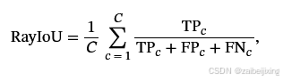
where TPc, FPc and FNc correspond to the number of true positive, false positive, and false negative predictions for class ci.
其中, TPc 、 FPc 和 FNc 分别对应类 ci 的真正例、假正例和假负例的数量。
RayIoU addresses all three of the aforementioned problems:
RayIoU 解决了上述所有三个问题:
-
Since the query ray calculates the distance to the first voxel it touches, the model cannot obtain a higher IoU by predicting a thicker surface.
- 由于查询射线计算的是它接触到的第一个体素的距离,因此模型无法通过预测更厚的表面来获得更高的 IoU。
-
RayIoU determines true positives based on a distance threshold, which mitigates the overly strict nature of voxel-level mIoU.
- RayIoU 通过基于距离阈值确定真实阳性来减轻体素级 mIoU 过于严格的特性。
-
The query ray can originate from any position in the scene. This flexibility allows RayIoU to consider the model's scene completion ability, preventing the reduction of occupancy estimation to mere depth prediction.
- 查询射线可以起源于场景中的任意位置。这种灵活性使 RayIoU 能够考虑模型的场景补全能力,防止将占用率估计简化为单纯的深度预测。
5 Experiments
5 实验
We evaluate our model on the Occ3D-nuScenes [50](https://arxiv.org/html/2312.17118v5#bib.bib50 "50") dataset. Occ3D-nuScenes is based on the nuScenes [3](https://arxiv.org/html/2312.17118v5#bib.bib3 "3") dataset, which consists of large-scale multimodal data collected from 6 surround-view cameras, 1 lidar and 5 radars. The dataset has 1000 videos in total and is split into 700/150/150 videos for training/validation/testing. Each video has roughly 20s duration and the key samples are annotated every 0.5s.
我们在 Occ3D-nuScenes 50数据集上评估我们的模型。Occ3D-nuScenes 基于 nuScenes 3数据集,该数据集由来自 6 个环绕视图相机、1 个激光雷达和 5 个雷达的大规模多模态数据组成。数据集总共包含 1000 个视频,并分为 700/150/150 个视频用于训练/验证/测试。每个视频的时长大约为 20 秒,关键样本每 0.5 秒进行一次标注。
We use the proposed RayIoU to evaluate the semantic segmentation performance. The query rays originate from 8 LiDAR positions of the ego path. We calculate RayIoU under three distance thresholds: 1, 2 and 4 meters. The final ranking metric is averaged over these distance thresholds.
我们使用所提出的 RayIoU 来评估语义分割性能。查询射线源自自车路径的 8 个 LiDAR 位置。我们在三个距离阈值下计算 RayIoU:1 米、2 米和 4 米。最终的排序指标在这些距离阈值上进行平均。
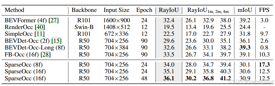
Table 1: 3D occupancy prediction performance on Occ3D-nuScenes [50](https://arxiv.org/html/2312.17118v5#bib.bib50 "50"). We use RayIoU to compare our SparseOcc with other methods. "8f" and "16f" mean fusing temporal information from 8 or 16 frames. SparseOcc outperforms all existing methods under a weaker setting.
表 1:在 Occ3D-nuScenes 50上的 3D 占有率预测性能。我们使用 RayIoU 来比较我们的 SparseOcc 与其他方法。"8f"和"16f"表示融合 8 或 16 帧的时间信息。在较弱的设置下,SparseOcc 优于所有现有方法。
5.1 Implementation Details
5.1 实现细节
We implement our model using PyTorch [41](https://arxiv.org/html/2312.17118v5#bib.bib41 "41"). Following previous methods, we adopt ResNet-50 [14](https://arxiv.org/html/2312.17118v5#bib.bib14 "14") as the image backbone. The mask transformer consists of 3 layers with shared weights across different layers. In our main experiments, we employ semantic queries where each query corresponds to a semantic class, rather than an instance. The ray casting module in RayIoU is implemented based on the codebase of [21](https://arxiv.org/html/2312.17118v5#bib.bib21 "21").
我们使用 PyTorch 41实现我们的模型。按照之前的方法,我们采用 ResNet-50 14作为图像主干。掩码变换器由 3 层组成,不同层之间共享权重。在我们的主要实验中,我们使用语义查询,每个查询对应一个语义类别,而不是一个实例。RayIoU 中的光线投射模块基于 21的代码库实现。
During training, we use the AdamW [36](https://arxiv.org/html/2312.17118v5#bib.bib36 "36") optimizer with a global batch size of 8. The initial learning rate is set to 2×10⁻⁴ and is decayed with cosine annealing policy. For all experiments, we train our models for 24 epochs. FPS is measured on a Tesla A100 GPU with the PyTorch fp32 backend.
在训练过程中,我们使用 AdamW 36优化器,全局批量大小为 8。初始学习率设置为 2×10⁻⁴ ,并使用余弦退火策略进行衰减。对于所有实验,我们训练模型 24 个周期。FPS 在 Tesla A100 GPU 上使用 PyTorch fp32 后端进行测量。
5.2 Main Results
5.2 主要结果
In Tab. 1 and Fig. 1 (b), we compare SparseOcc with previous state-of-the-art methods on the validation split of Occ3D-nuScenes. Despite under a weaker setting (ResNet-50 [14](https://arxiv.org/html/2312.17118v5#bib.bib14 "14"), 8 history frames, and input image resolution of 704 × 256), SparseOcc significantly outperforms previous methods including FB-Occ, the winner of CVPR 2023 occupancy challenge, with many complicated designs including forward-backward view transformation, depth net, joint depth and semantic pre-training, and so on. SparseOcc achieves better results (+1.6 RayIoU) while being much faster and simpler than FB-Occ, which demonstrates the superiority of our solution.
在表 1 和图 1(b)中,我们将 SparseOcc 与 Occ3D-nuScenes 验证集上的先前最先进方法进行了比较。尽管在较弱的设置下(ResNet-50 14,8 个历史帧,输入图像分辨率为 704 × 256),SparseOcc 仍然显著优于先前的方法,包括 FB-Occ,CVPR 2023 占用率挑战赛的获胜者,后者具有许多复杂设计,如前向-后向视图转换、深度网络、联合深度和语义预训练等。SparseOcc 在取得更好结果(+1.6 RayIoU)的同时,比 FB-Occ 更快更简单,这证明了我们解决方案的优越性。
We further provide qualitative results in Fig. 7. Both BEVDet-Occ and FB-Occ are dense methods and make many redundant predictions behind the surface. In contrast, SparseOcc discards over 90% of voxels while still effectively modeling the geometry of the scene and capturing fine-grained details.
我们在图 7 中进一步提供了定性结果。BEVDet-Occ 和 FB-Occ 都是密集方法,在表面后面做出了许多冗余预测。相比之下,SparseOcc 丢弃了超过 90%的体素,同时仍然有效地建模场景的几何形状并捕捉细粒度细节。
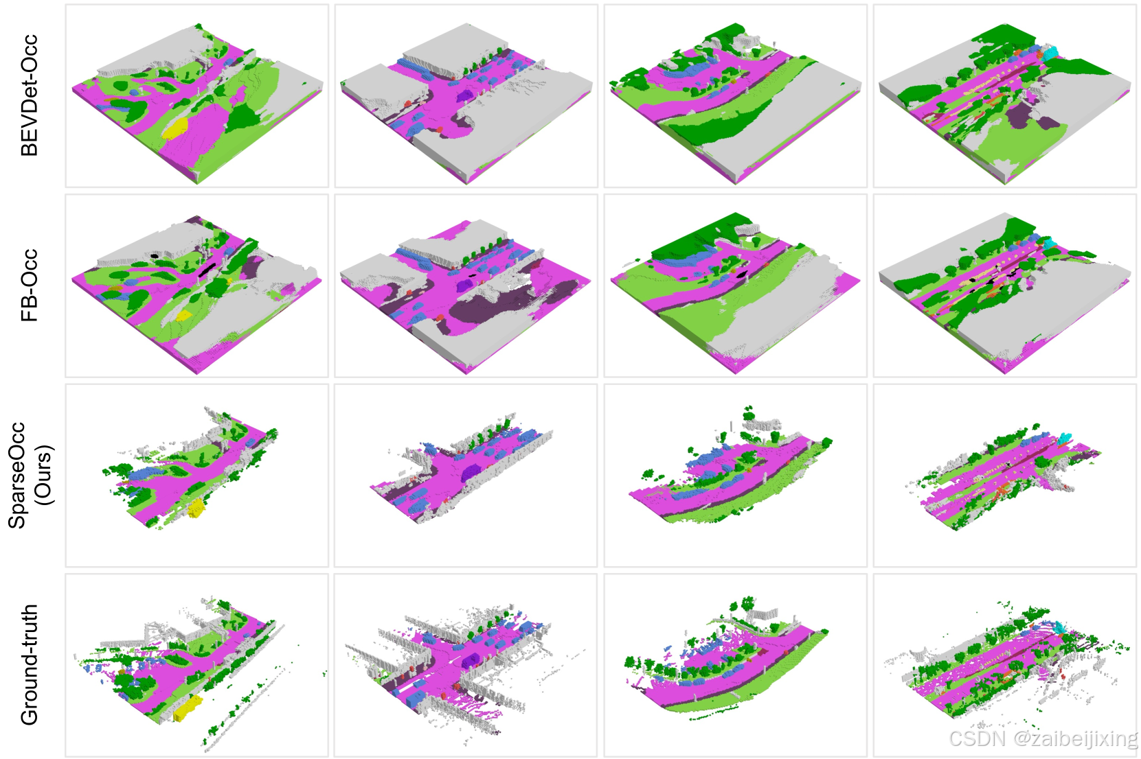
(a) (1) Figure 7: Visualized comparison of semantic occupancy prediction. Despite discarding over 90% of voxels, our SparseOcc effectively models the geometry of the scene and captures fine-grained details (e.g ., the yellow-marked traffic cone in the bottom row).
图 7:语义占有率预测的可视化比较。尽管丢弃了超过 90%的体素,我们的 SparseOcc 仍能有效建模场景的几何形状,并捕捉精细细节(例如,底部行中用黄色标记的交通锥)。
5.3 Ablations
5.3 消融研究
In this section, we conduct ablations on the validation split of Occ3D-nuScenes to confirm the effectiveness of each module. By default, we use the single frame version of SparseOcc as the baseline. The choice for our model is made bold.
在本节中,我们对 Occ3D-nuScenes 的验证集进行消融实验,以确认每个模块的有效性。默认情况下,我们使用 SparseOcc 的单帧版本作为基线。我们的模型选择以粗体显示。
Table 2: Sparse voxel decoder vs. dense voxel decoder. Our sparse voxel decoder achieves nearly 4× faster inference speed than the dense counterparts.
表 2:稀疏体素解码器与密集体素解码器的对比。我们的稀疏体素解码器在推理速度上比密集体素解码器快近 4 倍。

Sparse voxel decoder vs. dense voxel decoder.
稀疏体素解码器 vs. 密集体素解码器。
In Tab. 2, we compare our sparse voxel decoder to the dense counterparts. Here, we implement two baselines, and both of them output a dense feature map with shape as 200×200×16×C. The first baseline is a coarse-to-fine architecture without pruning empty voxels. In this baseline, we also replace self-attention with 3D convolution and use 3D deconvolution to upsample predictions. The other baseline is a patch-based architecture by dividing the 3D space into a small number of patches as PETRv2 [35](https://arxiv.org/html/2312.17118v5#bib.bib35 "35") for BEV segmentation. We use 25×25×2 = 1250 queries and each one of them corresponds to a specific patch of shape 8×8×8. A stack of deconvolution layers are used to lift the coarse queries to a full-resolution 3D volume.
在表 2 中,我们将我们的稀疏体素解码器与密集的对应物进行了比较。在这里,我们实现了两个基线,它们都输出一个形状为 200 × 200 × 16 × C 的密集特征图。第一个基线是一个从粗到细的架构,没有修剪空体素。在这个基线中,我们还将自注意力替换为 3D 卷积,并使用 3D 反卷积来上采样预测。另一个基线是基于补丁的架构,通过将 3D 空间划分为少量补丁,类似于 PETRv2 35用于 BEV 分割。我们使用 25 × 25 × 2 = 1250 个查询,每个查询对应一个特定形状为 8 × 8 × 8 的补丁。一系列反卷积层用于将粗略的查询提升到全分辨率的 3D 体积。
As we can see from the table, the dense coarse-to-fine baseline achieves a good performance of 29.9 RayIoU but with a slow inference speed of 6.3 FPS. The patch-based one is slightly faster with 7.8 FPS inference speed but with a severe performance drop by 4.1 RayIoU. Instead, our sparse voxel decoder produces sparse 3D features in the shape of K×C (where K = 32000 ≪ 200×200×16), achieving an inference speed that is nearly 4× faster than the counterparts without compromising performance. This demonstrates the necessity and effectiveness of our sparse design.
从表格中可以看出,密集的粗到细基线实现了 29.9 RayIoU 的良好性能,但推理速度较慢,为 6.3 FPS。基于补丁的方法稍快,推理速度为 7.8 FPS,但性能严重下降了 4.1 RayIoU。相反,我们的稀疏体素解码器在形状为 K×C (其中 K =32000 ≪ 200 × 200 × 16)的情况下生成稀疏的 3D 特征,推理速度几乎比同类产品快 4 × ,同时不牺牲性能。这证明了我们稀疏设计的必要性和有效性。
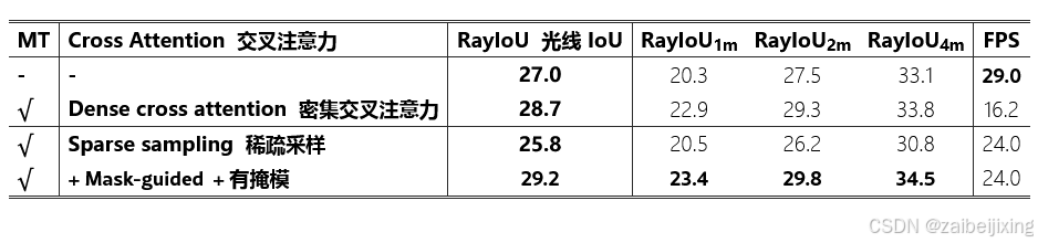
Table 3: Ablation of mask transformer (MT) and the cross attention module in MT. Mask-guided sparse sampling is stronger and faster than the dense cross attention.
表 3:对掩码变换器(MT)及其交叉注意力模块的消融研究。基于掩码的稀疏采样比密集交叉注意力更强大且更高效。
Mask Transformer.
掩码变换器。
In Tab. 3, we ablate the effectiveness of the mask transformer. The first row is a simple per-voxel baseline which directly predicts semantics from the sparse voxel decoder using a stack of MLPs. Introducing mask transformer with vanilla cross attention (as it is the common practice in MaskFormer and Mask3D) gives a performance boost of 1.7 RayIoU, but inevitably slows down the inference speed as it attends to all locations in an image. Therefore, to speed up the dense cross-attention pipeline, we adopt a sparse sampling mechanism which brings a 50% reduction in inference time. By further introducing the predicted masks to guide the generation of sampling points, we finally achieve 29.2 RayIoU with 24 FPS.
在表 3 中,我们对掩码变换器的有效性进行了消融研究。第一行是一个简单的逐体素基线,它直接使用一系列 MLP 从稀疏体素解码器预测语义。引入具有普通交叉注意力的掩码变换器(因为在 MaskFormer 和 Mask3D 中这是常见的做法)可以提高 1.7 RayIoU 的性能,但不可避免地会减慢推理速度,因为它会关注图像中的所有位置。因此,为了加快密集交叉注意力管道的速度,我们采用了一种稀疏采样机制,使推理时间减少了 50%。通过进一步将预测的掩码引入到采样点的生成中,我们最终实现了 29.2 RayIoU 的精度,同时以 24 FPS 的速度运行。
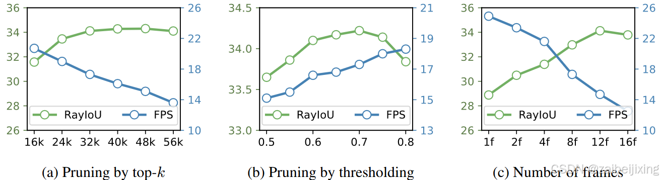
Figure 8: Ablations on voxel sparsity and temporal modeling. (a) The optimal performance occurs when k is set to 32000 (5% sparsity). (b) Top-k can also be substituted with thresholding, e.g ., voxels scoring less than a certain threshold will be pruned. (c) The performance continues to increase with the number of frames, but it starts to saturate after 12 frames.
图 8:对体素稀疏性和时间建模的消融研究。(a)当 k 设置为 32000(5%稀疏度)时,最佳性能出现。(b)顶部的 k 也可以用阈值代替,例如,得分低于某个阈值的体素将被修剪。(c)性能随着帧数的增加而继续提高,但在 12 帧后开始趋于饱和。
Is a limited set of voxels sufficient to cover the scene?
是否一个有限的体素集就足以覆盖整个场景?
In this study, we delve deeper into the impact of voxel sparsity on final performance. To investigate this, we systematically ablate the value of k in Fig. 8 (a). Starting from a modest value of 16k, we observe that the optimal performance occurs when k is set to 32k ∼ 48k, which is only 5% ∼ 7.5% of the total number of dense voxels (200×200×16 = 640000). Surprisingly, further increasing k does not yield any performance improvements; instead, it introduces noise. Thus, our findings suggest that a ∼5% sparsity level is sufficient. Keep increasing the density will reduce both accuracy and speed.
在本研究中,我们深入探讨了体素稀疏性对最终性能的影响。为了研究这一点,我们系统地消融了图 8(a)中的 k 值。从一个适中的 16k 值开始,我们观察到当 k 设置为 32k ∼ 48k 时,性能最优,这仅占总密集体素数的 5% ∼ 7.5%(200 × 200 × 16 = 640000)。令人惊讶的是,进一步增加 k 并没有带来任何性能提升,反而引入了噪声。因此,我们的研究结果表明, ∼ 5%的稀疏水平已经足够。继续增加密度将降低准确性和速度。
Pruning by top-k is simple and effective, but it is related to specific dataset. In real world, we can substitute top-k with a thresholding method. Voxels scoring less than a given threshold (e.g ., 0.7) will be pruned. Thresholding achieves similar performance to top-k (see Fig. 8 (b)), and has the ability to generalize to different scenes.
剪枝通过top-k 简单有效,但与特定数据集相关。在现实世界中,我们可以用阈值方法替代top-k 。得分小于给定阈值(例如,0.7)的体素将被剪枝。阈值方法实现了与top-k类似的性能(参见图 8 (b)),并且能够泛化到不同的场景。
Temporal modeling.
时间建模。
In Fig. 8 (c), we validate the effectiveness of temporal fusion. We can see that the temporal modeling of SparseOcc is very effective, with performance steadily increasing as the number of frames increases. The performance peaks at 12 frames and then saturates. However, the inference speed drops rapidly as the sampling points need to interact with every frame.
在图 8(c)中,我们验证了时间融合的有效性。我们可以看到 SparseOcc 的时间建模非常有效,随着帧数的增加,性能稳步提升。性能在 12 帧时达到峰值,然后饱和。然而,推理速度会迅速下降,因为采样点需要与每一帧进行交互。
5.4 More Studies
5.4 更多研究
Table 4: To verify the effect of the visible mask, wo provide per-class RayIoU of BEVFormer and FB-Occ. † uses the visible mask during training. We find that training with the visible mask hurts the performance of background classes such as drivable surface, terrian and sidewalk.
表 4:为了验证可见掩码的效果,我们提供了 BEVFormer 和 FB-Occ 的每类 RayIoU。 † 在训练中使用了可见掩码。我们发现使用可见掩码进行训练会损害背景类(如可行驶表面、地形和人行道)的性能。
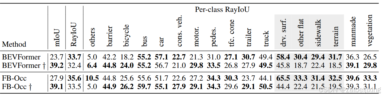
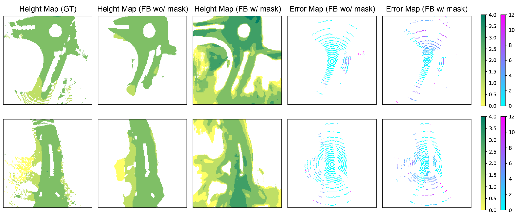
Figure 9: Why does the performance of background classes, such as drivable surfaces, degrade when using the visible mask during training? We provide a visualization of the drivable surface as predicted by FB-Occ. Here, "FB w/ mask" and "FB wo/ mask" denote training with and without the visible mask, respectively. We observe that "FB w/ mask" tends to predict a higher and thicker road surface, resulting in significant depth errors along a ray. In contrast, "FB wo/ mask" predicts a road surface that is both accurate and consistent.
图 9:为什么在训练中使用可见掩膜时,背景类(如可行驶表面)的性能会下降?我们提供了 FB-Occ 预测的可行驶表面的可视化。这里,"FB w/ mask"和"FB wo/ mask"分别表示使用和不使用可见掩膜进行训练。我们观察到,"FB w/ mask"倾向于预测更高更厚的路面,导致沿射线的深度误差显著。相比之下,"FB wo/ mask"预测的路面既准确又一致。
The effect of training with visible masks.
使用可见掩码进行训练的效果。
Interestingly, we observed a peculiar phenomenon. Under the traditional voxel-level mIoU metric, dense methods can significantly benefit from disregarding the non-visible voxels during training. These non-visible voxels are indicated by a binary visible mask provided by the Occ3D-nuScenes dataset. However, we find that this strategy actually impairs performance under our new RayIoU metric. For instance, we train two variants of BEVFormer: one uses the visible mask during training, and the other does not. As shown in Tab. 4, the former scores 15 points higher than the latter on the voxel-based mIoU, but it scores 1 point lower on RayIoU. This phenomenon is also observed on FB-Occ.
有趣的是,我们观察到一个奇特的现象。在传统的体素级 mIoU 指标下,密集方法在训练过程中忽略非可见体素时可以显著受益。这些非可见体素由 Occ3D-nuScenes 数据集提供的二值可见性掩膜指示。然而,我们发现这一策略在我们的新 RayIoU 指标下反而损害了性能。例如,我们训练了 BEVFormer 的两个变体:一个在训练中使用可见性掩膜,另一个不使用。如表 4 所示,前者在基于体素的 mIoU 上比后者高 15 分,但在 RayIoU 上低 1 分。这一现象也在 FB-Occ 上观察到。
To further explore this, we present the per-class RayIoU in Tab. 4. The table reveals that training with the visible mask enhances performance for most foreground classes such as bus, bicycle, and truck. However, it negatively impacts background classes like drivable surface and terrain.
为了进一步探讨这个问题,我们在表 4 中展示了每类的 RayIoU。该表显示,使用可见掩码进行训练可以提高大多数前景类(如公共汽车、自行车和卡车)的性能。然而,它对可行驶表面和地形等背景类产生了负面影响。
This observation raises a further question: Why does the performance of the background category degrade? To address this, we offer a visual comparison of the depth errors and height maps of the predicted drivable surface from FB-Occ in Fig. 9, both with and without the use of visible mask during training. The figure illustrates that training with visible masks results in a thicker and higher ground prediction, leading to substantial depth errors in distant areas. Conversely, models trained without the visible mask predict depth with greater accuracy.
这一观察提出了一个进一步的问题:为什么背景类别的性能会下降?为了解决这个问题,我们在图 9 中提供了一个视觉比较,比较了 FB-Occ 预测的可行驶表面的深度误差和高度图,分别使用了可见掩码和未使用可见掩码进行训练。该图表明,使用可见掩码进行训练会导致预测的地面更厚、更高,从而在远距离区域产生显著的深度误差。相反,未使用可见掩码训练的模型在预测深度时具有更高的准确性。
From these observations, we derive some valuable insights: ignoring non-visible voxels during training benefits foreground classes by resolving the issue of ambiguous labeling of unscanned voxels. However, it also compromises the accuracy of depth estimation, as models tend to predict a thicker and closer surface. We hope that our findings will benefit future research.
从这些观察中,我们得出了一些有价值的见解:在训练过程中忽略非可见体素有助于前景类别,通过解决未扫描体素的模糊标记问题。然而,它也损害了深度估计的准确性,因为模型倾向于预测更厚和更近的表面。我们希望我们的研究结果将对未来的研究有所帮助。
Panoptic occupancy.
全景占用。
We then show that SparseOcc can be easily extended for panoptic occupancy prediction, a task derived from panoptic segmentation that segments images to not only semantically meaningful regions but also to detect and distinguish individual instances. Compared to panoptic segmentation, panoptic occupancy prediction requires the model to have geometric awareness in order to construct the 3D scene for segmentation. By additionally introducing instance queries to the mask transformer, we seamlessly achieve the first fully sparse panoptic occupancy prediction framework using camera-only inputs.
我们随后展示了 SparseOcc 可以轻松扩展用于全景占用预测,这是从全景分割派生的任务,该任务将图像分割为不仅具有语义意义的区域,还能够检测和区分单个实例。与全景分割相比,全景占用预测要求模型具有几何意识,以便为分割构建 3D 场景。通过额外引入实例查询到掩码变换器,我们无缝地实现了第一个完全稀疏的全景占用预测框架,仅使用相机输入。
Firstly, we utilize the ground-truth bounding boxes from the 3D object detection task to generate the panoptic occupancy ground truth. Specifically, we define eight instance categories (including car, truck, construction vehicle, bus, trailer, motorcycle, bicycle, pedestrian) and ten staff categories (including terrain, manmade, vegetation, etc). Each instance segment is identified by grouping the voxels inside the bounding box based on an existing semantic occupancy benchmark, such as Occ3D-nuScenes.
首先,我们利用 3D 物体检测任务中的地面真实边界框来生成全景占用地面真值。具体而言,我们定义了八个实例类别(包括汽车、卡车、施工车辆、公共汽车、拖车、摩托车、自行车和行人)和十个设施类别(包括地形、人造、植被等)。每个实例分割是通过根据现有的语义占用基准(如 Occ3D-nuScenes)对边界框内的体素进行分组来识别的。
We then design RayPQ based on the well-known panoptic quality (PQ) [22](https://arxiv.org/html/2312.17118v5#bib.bib22 "22") metric, which is defined as the multiplication of segmentation quality (SQ) and recognition quality (RQ):
我们随后基于著名的全景质量(PQ)22指标设计了 RayPQ,该指标被定义为分割质量(SQ)和识别质量(RQ)的乘积:
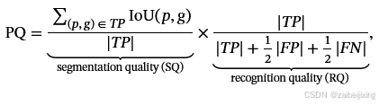
where the definition of true positive (TP) is the same as that in RayIoU. The threshold of IoU between prediction p and ground-truth g is set to 0.5.
在 RayIoU 中,真阳性(TP)的定义与此相同。预测 p 和真实值 g 之间的 IoU 阈值设置为 0.5。
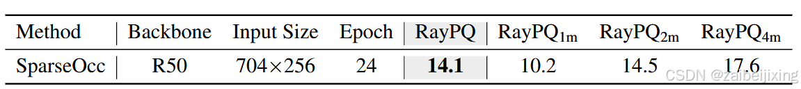
Table 5: Panoptic occupancy prediction performance on Occ3D-nuScenes.
表 5:Occ3D-nuScenes 上的全景占用预测性能。
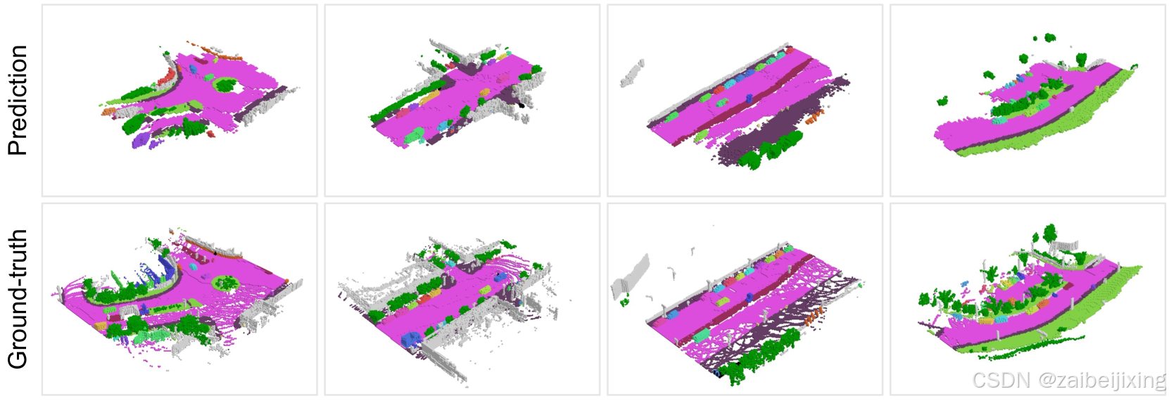
(a) (1) Figure 10: Panoptic occupancy prediction. Different instances are distinguished by colors. Our model can capture fine-grained objects and road structures simultaneously.
图 10:全景占用预测。不同的实例通过颜色区分。我们的模型可以同时捕捉细粒度的对象和道路结构。
In Tab. 5, we report the performance of SparseOcc on panoptic occupancy benchmark. Similar to RayIoU, we calculate RayPQ under three distance thresholds: 1, 2 and 4 meters. SparseOcc achieves an averaged RayPQ of 14.1. The visualizations are presented in Fig. 10.
在表 5 中,我们报告了 SparseOcc 在全景占用基准上的性能。与 RayIoU 类似,我们在三个距离阈值下计算 RayPQ:1 米、2 米和 4 米。SparseOcc 实现了平均 RayPQ 为 14.1。可视化结果如图 10 所示。
5.5 Limitations
5.5 限制
Accumulative errors.
累积误差。
In order to implement a fully sparse architecture, we discard a large number of empty voxels in the early stages. However, empty voxels that are mistakenly discarded cannot be recovered in subsequent stages. Moreover, the prediction of the mask transformer is constrained within a space predicted by the sparse voxel decoder. Some ground-truth instances do not appear in this unreliable space, leading to inadequate training of the mask transformer.
为了实现完全稀疏架构,我们在早期阶段丢弃了大量空体素。然而,被错误丢弃的空体素在后续阶段无法恢复。此外,掩码变换器的预测被限制在稀疏体素解码器预测的空间内。一些真实实例不出现在这个不可靠的空间中,导致掩码变换器的训练不足。
6 Conclusion
6 结论
In this paper, we proposed a fully sparse occupancy network, named SparseOcc, which neither relies on dense 3D feature, nor has sparse-to-dense and global attention operations. We also created RayIoU, a ray-level metric for occupancy evaluation, eliminating the inconsistency flaws of previous metric. Experiments show that SparseOcc achieves the state-of-the-art performance on the Occ3D-nuScenes dataset for both speed and accuracy. We hope this exciting result will attract more attention to the fully sparse 3D occupancy paradigm.
在本文中,我们提出了一种完全稀疏的占用网络,名为 SparseOcc,它既不依赖于密集的 3D 特征,也不涉及从稀疏到密集和全局注意力操作。我们还创建了 RayIoU,这是一种用于占用评估的射线级指标,消除了先前指标的不一致缺陷。实验表明,SparseOcc 在 Occ3D-nuScenes 数据集上实现了速度和准确性方面的最新性能。我们希望这一令人兴奋的结果将吸引更多关注完全稀疏的 3D 占用范式。
Acknowledgements
致谢
We thank the anonymous reviewers for their suggestions that make this work better. This work is supported by the National Key R&D Program of China (No. 2022ZD0160900), the National Natural Science Foundation of China (No. 62076119, No. 61921006), the Fundamental Research Funds for the Central Universities (No. 020214380119), and the Collaborative Innovation Center of Novel Software Technology and Industrialization.
我们感谢匿名审稿人的建议,使这项工作变得更好。这项工作得到了中国国家重点研发计划(No. 2022ZD0160900)、国家自然科学基金(No. 62076119, No. 61921006)、中央高校基本科研业务费专项资金(No. 020214380119)以及国家示范性软件学院联合创新中心的支持。
声明:本文主要取材于ar5iv,本人对全文中文翻译部分进行了细致全面的校验和编辑工作。