Day 13 编程实战:朴素贝叶斯与极端涨跌预警
实战目标
- 理解朴素贝叶斯的原理和独立假设
- 掌握三种朴素贝叶斯模型的使用
- 实现极端涨跌预警(5档分类)
- 对比不同朴素贝叶斯模型的效果
1. 导入必要的库
python
import numpy as np
import pandas as pd
import matplotlib.pyplot as plt
import seaborn as sns
import time
from pathlib import Path
from sklearn.naive_bayes import GaussianNB, MultinomialNB, BernoulliNB
from sklearn.preprocessing import StandardScaler, MinMaxScaler, KBinsDiscretizer
from sklearn.model_selection import train_test_split, TimeSeriesSplit, cross_val_score
from sklearn.metrics import (
    accuracy_score, precision_score, recall_score, f1_score,
    confusion_matrix, classification_report, ConfusionMatrixDisplay
)
from sklearn.datasets import make_classification
import warnings
warnings.filterwarnings('ignore')

sns.set_style("whitegrid")  # 预设样式
#启用LaTeX渲染(如果系统安装了LaTeX)
plt.rcParams['text.usetex'] = False  # 设为False避免LaTeX依赖
# 设置中文显示
plt.rcParams['font.sans-serif'] = ['Microsoft YaHei', 'DejaVu Sans']
plt.rcParams['axes.unicode_minus'] = False
plt.rcParams['mathtext.fontset'] = 'dejavusans'  # 或 'stix'
2. 朴素贝叶斯原理可视化
2.1 贝叶斯定理可视化
可视化贝叶斯定理的核心公式:
P(Y∣X1,X2)=P(X1∣Y)⋅P(X2∣Y)⋅P(Y)P(X1,X2) P(Y|X_1, X_2) = \frac{P(X_1|Y) \cdot P(X_2|Y) \cdot P(Y)}{P(X_1, X_2)} P(Y∣X1,X2)=P(X1,X2)P(X1∣Y)⋅P(X2∣Y)⋅P(Y)
朴素假设:
P(X1,X2∣Y)=P(X1∣Y)⋅P(X2∣Y) P(X_1, X_2|Y) = P(X_1|Y) \cdot P(X_2|Y) P(X1,X2∣Y)=P(X1∣Y)⋅P(X2∣Y)
其中:
- P(Y∣X1,X2)P(Y|X_1, X_2)P(Y∣X1,X2):后验概率(我们想要预测的)
- P(X1∣Y),P(X2∣Y)P(X_1|Y),P(X_2|Y)P(X1∣Y),P(X2∣Y):似然函数(给定类别下观察到特征的概率)
- P(Y)P(Y)P(Y):先验概率(类别的基础概率)
- P(X1,X2)P(X_1, X_2)P(X1,X2) :证据(特征出现的总概率)
python
def visualize_bayes_theorem():
    """可视化贝叶斯定理"""
    # 模拟数据
    np.random.seed(42)  # 确保结果可重现
    n_samples = 1000    # 样本总数

    # 定义类别和特征
    # 2个类别:0(负类)和 1(正类)
    # 2个特征:feature1 和 feature2
    class_probs = [0.7, 0.3]  # 类别先验概率 P(C0)=0.7, P(C1)=0.3

    # 生成类别标签
    y = np.random.choice([0, 1], size=n_samples, p=class_probs)

    # 为每个类别生成特征数据(朴素贝叶斯假设特征独立)
    # 类别0:feature1 ~ N(2, 1), feature2 ~ N(2, 1)
    # 类别1:feature1 ~ N(4, 1), feature2 ~ N(4, 1)
    X = np.zeros((n_samples, 2))

    for i in range(n_samples):
        if y[i] == 0:  # 类别0
            X[i, 0] = np.random.normal(2, 1)  # feature1
            X[i, 1] = np.random.normal(2, 1)  # feature2
        else:  # 类别1
            X[i, 0] = np.random.normal(4, 1)  # feature1
            X[i, 1] = np.random.normal(4, 1)  # feature2

    # 创建可视化
    fig, axes = plt.subplots(2, 2, figsize=(15, 12))

    # 1. 散点图:显示两类数据的分布
    scatter = axes[0, 0].scatter(X[y == 0, 0], X[y == 0, 1],
                                c='blue', alpha=0.6, label='类别 0', s=30)
    axes[0, 0].scatter(X[y == 1, 0], X[y == 1, 1],
                      c='red', alpha=0.6, label='类别 1', s=30)
    axes[0, 0].set_xlabel('特征 1')
    axes[0, 0].set_ylabel('特征 2')
    axes[0, 0].set_title('数据分布\n(蓝色=类别0, 红色=类别1)')
    axes[0, 0].legend()
    axes[0, 0].grid(True, alpha=0.3)

    # 2. 特征1的条件分布 P(X1|Y)
    x1_range = np.linspace(0, 6, 200)
    # 类别0的feature1分布
    p_x1_given_c0 = (1/np.sqrt(2*np.pi*1)) * np.exp(-0.5*((x1_range-2)**2)/1)
    # 类别1的feature1分布
    p_x1_given_c1 = (1/np.sqrt(2*np.pi*1)) * np.exp(-0.5*((x1_range-4)**2)/1)

    axes[0, 1].plot(x1_range, p_x1_given_c0, 'b-', linewidth=2, label='P(X1|C0)')
    axes[0, 1].plot(x1_range, p_x1_given_c1, 'r-', linewidth=2, label='P(X1|C1)')
    axes[0, 1].set_xlabel('特征 1')
    axes[0, 1].set_ylabel('概率密度')
    axes[0, 1].set_title('条件概率 P(X1|Y)')
    axes[0, 1].legend()
    axes[0, 1].grid(True, alpha=0.3)

    # 3. 特征2的条件分布 P(X2|Y)
    x2_range = np.linspace(0, 6, 200)
    # 类别0的feature2分布
    p_x2_given_c0 = (1/np.sqrt(2*np.pi*1)) * np.exp(-0.5*((x2_range-2)**2)/1)
    # 类别1的feature2分布
    p_x2_given_c1 = (1/np.sqrt(2*np.pi*1)) * np.exp(-0.5*((x2_range-4)**2)/1)

    axes[1, 0].plot(x2_range, p_x2_given_c0, 'b-', linewidth=2, label='P(X2|C0)')
    axes[1, 0].plot(x2_range, p_x2_given_c1, 'r-', linewidth=2, label='P(X2|C1)')
    axes[1, 0].set_xlabel('特征 2')
    axes[1, 0].set_ylabel('概率密度')
    axes[1, 0].set_title('条件概率 P(X2|Y)')
    axes[1, 0].legend()
    axes[1, 0].grid(True, alpha=0.3)

    # 4. 后验概率 P(Y|X1, X2) 的可视化
    # 创建网格
    x1_mesh, x2_mesh = np.meshgrid(np.linspace(0, 6, 100), np.linspace(0, 6, 100))

    # 计算 P(X1, X2|C0) * P(C0)
    p_x1_given_c0_mesh = (1/np.sqrt(2*np.pi*1)) * np.exp(-0.5*((x1_mesh-2)**2)/1)
    p_x2_given_c0_mesh = (1/np.sqrt(2*np.pi*1)) * np.exp(-0.5*((x2_mesh-2)**2)/1)
    numerator_c0 = p_x1_given_c0_mesh * p_x2_given_c0_mesh * class_probs[0]  # P(X1,X2|C0) * P(C0)

    # 计算 P(X1, X2|C1) * P(C1)
    p_x1_given_c1_mesh = (1/np.sqrt(2*np.pi*1)) * np.exp(-0.5*((x1_mesh-4)**2)/1)
    p_x2_given_c1_mesh = (1/np.sqrt(2*np.pi*1)) * np.exp(-0.5*((x2_mesh-4)**2)/1)
    numerator_c1 = p_x1_given_c1_mesh * p_x2_given_c1_mesh * class_probs[1]  # P(X1,X2|C1) * P(C1)

    # 归一化得到后验概率
    denominator = numerator_c0 + numerator_c1
    p_c0_given_x = numerator_c0 / denominator
    p_c1_given_x = numerator_c1 / denominator

    # 绘制后验概率热图
    im = axes[1, 1].contourf(x1_mesh, x2_mesh, p_c1_given_x, levels=20, cmap='RdYlBu_r', alpha=0.8)
    contour = axes[1, 1].contour(x1_mesh, x2_mesh, p_c1_given_x, levels=[0.5], colors='black', linewidths=2)
    axes[1, 1].clabel(contour, inline=True, fontsize=10, fmt={0.5: '决策边界'})

    # 添加样本点
    axes[1, 1].scatter(X[y == 0, 0], X[y == 0, 1], c='blue', alpha=0.6, label='类别 0', s=30)
    axes[1, 1].scatter(X[y == 1, 0], X[y == 1, 1], c='red', alpha=0.6, label='类别 1', s=30)

    axes[1, 1].set_xlabel('特征 1')
    axes[1, 1].set_ylabel('特征 2')
    axes[1, 1].set_title('后验概率 P(C1|X1, X2)\n(颜色深浅表示概率大小)')
    axes[1, 1].legend()

    # 添加颜色条
    cbar = plt.colorbar(im, ax=axes[1, 1])
    cbar.set_label('P(C1|X1, X2)')

    plt.tight_layout()
    plt.show()

    # 打印一些统计信息
    print(f"类别分布: 类别0占比 {np.mean(y==0):.2f}, 类别1占比 {np.mean(y==1):.2f}")
    print(f"先验概率: P(C0)={class_probs[0]}, P(C1)={class_probs[1]}")
    print(f"特征1均值 - C0: {np.mean(X[y==0, 0]):.2f}, C1: {np.mean(X[y==1, 0]):.2f}")
    print(f"特征2均值 - C0: {np.mean(X[y==0, 1]):.2f}, C1: {np.mean(X[y==1, 1]):.2f}")

# 调用函数进行可视化
visualize_bayes_theorem()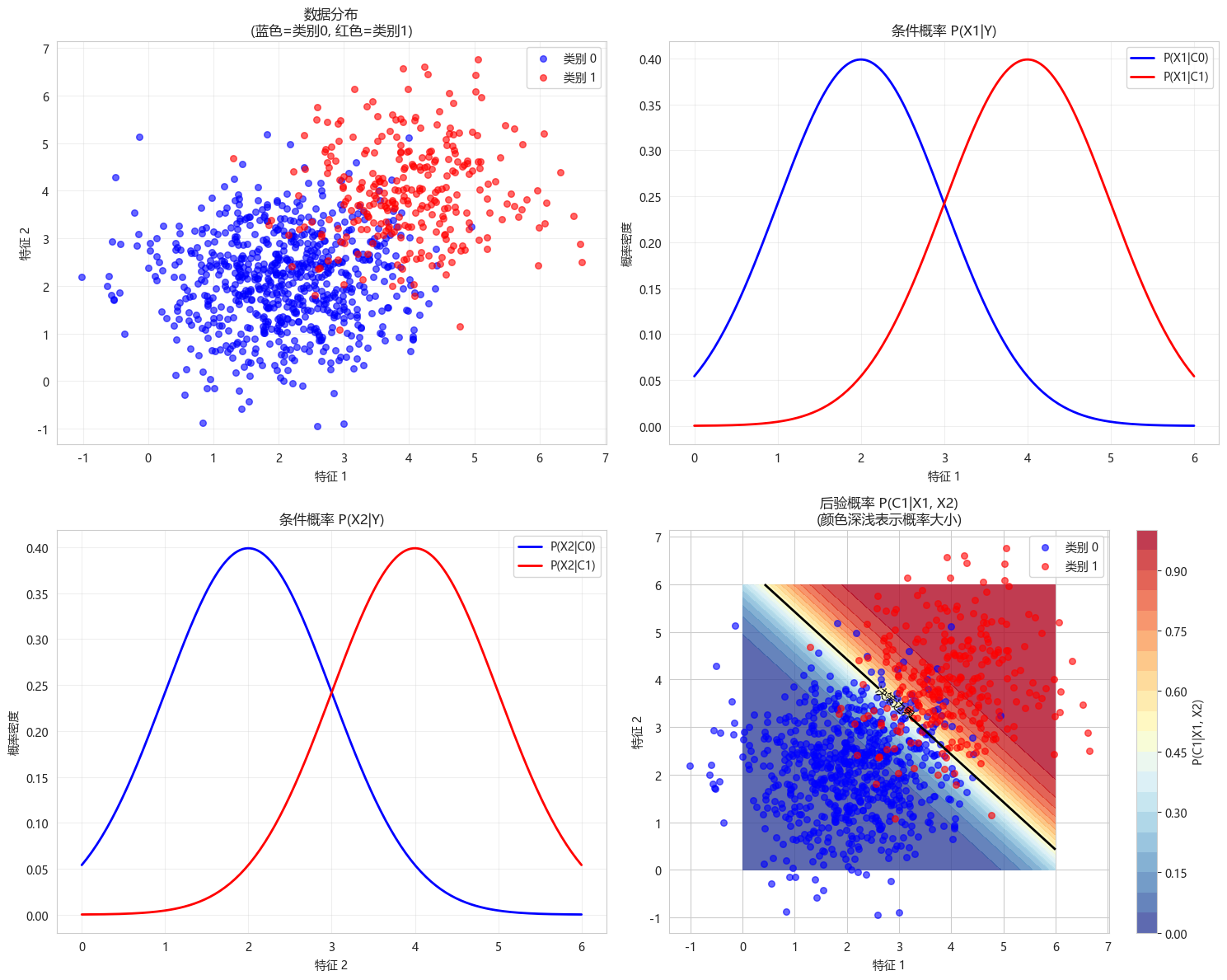
类别分布: 类别0占比 0.71, 类别1占比 0.29
先验概率: P(C0)=0.7, P(C1)=0.3
特征1均值 - C0: 2.06, C1: 4.01
特征2均值 - C0: 2.11, C1: 3.97
四个子图的含义:
-
左上角:数据分布
- 展示两个类别的二维数据点
- 验证朴素贝叶斯的假设:特征在类别内呈高斯分布
-
右上角:P(X1∣Y)P(X_1|Y)P(X1∣Y)
- 条件概率分布
- 展示给定类别下特征1的分布
-
左下角:P(X2∣Y)P(X_2|Y)P(X2∣Y)
- 条件概率分布
- 展示给定类别下特征2的分布
-
右下角:P(Y∣X1,X2)P(Y|X_1, X_2)P(Y∣X1,X2)
- 核心:后验概率热图
- 黑色线:决策边界(P(C1∣X)=0.5P(C_1|X)=0.5P(C1∣X)=0.5)
- 颜色深浅:属于类别1的概率
2.2 特征独立性假设演示
python
def visualize_independence_assumption():
    """演示特征独立假设的影响"""
    np.random.seed(42)
    n_samples = 500

    # 生成相关特征
    mean = [0, 0]
    cov = [[1, 0.8], [0.8, 1]]  # 协方差矩阵(高度相关)
    # 生成多元高斯分布(多维正态分布)随机样本
    X_correlated = np.random.multivariate_normal(mean, cov, n_samples)
    y = (X_correlated[:, 0] + X_correlated[:, 1] > 0).astype(int)

    # 生成独立特征
    X_independent = np.random.randn(n_samples, 2)
    y_indep = (X_independent[:, 0] + X_independent[:, 1] > 0).astype(int)

    fig, axes = plt.subplots(2, 2, figsize=(12, 10))

    # 相关特征散点图
    axes[0, 0].scatter(X_correlated[y == 0, 0], X_correlated[y == 0, 1],
                       c='blue', alpha=0.5, label='下跌')
    axes[0, 0].scatter(X_correlated[y == 1, 0], X_correlated[y == 1, 1],
                       c='red', alpha=0.5, label='上涨')
    axes[0, 0].set_xlabel('特征1')
    axes[0, 0].set_ylabel('特征2')
    axes[0, 0].set_title('相关特征(相关性=0.8)')
    axes[0, 0].legend()
    axes[0, 0].grid(True, alpha=0.3)

    # 独立特征散点图
    axes[0, 1].scatter(X_independent[y_indep == 0, 0], X_independent[y_indep == 0, 1],
                       c='blue', alpha=0.5, label='下跌')
    axes[0, 1].scatter(X_independent[y_indep == 1, 0], X_independent[y_indep == 1, 1],
                       c='red', alpha=0.5, label='上涨')
    axes[0, 1].set_xlabel('特征1')
    axes[0, 1].set_ylabel('特征2')
    axes[0, 1].set_title('独立特征')
    axes[0, 1].legend()
    axes[0, 1].grid(True, alpha=0.3)

    # 训练高斯朴素贝叶斯
    gnb_corr = GaussianNB()
    gnb_corr.fit(X_correlated, y)
    gnb_indep = GaussianNB()
    gnb_indep.fit(X_independent, y_indep)

    # 决策边界
    x_min, x_max = -3, 3
    y_min, y_max = -3, 3
    xx, yy = np.meshgrid(np.arange(x_min, x_max, 0.05),
                         np.arange(y_min, y_max, 0.05))

    Z_corr = gnb_corr.predict(np.c_[xx.ravel(), yy.ravel()])
    Z_corr = Z_corr.reshape(xx.shape)
    axes[1, 0].contourf(xx, yy, Z_corr, alpha=0.3, cmap='RdYlBu')
    axes[1, 0].scatter(X_correlated[y == 0, 0], X_correlated[y == 0, 1],
                       c='blue', alpha=0.5, s=20)
    axes[1, 0].scatter(X_correlated[y == 1, 0], X_correlated[y == 1, 1],
                       c='red', alpha=0.5, s=20)
    axes[1, 0].set_title(f'相关特征 - 高斯NB\n准确率: {gnb_corr.score(X_correlated, y):.3f}')
    axes[1, 0].set_xlabel('特征1')
    axes[1, 0].set_ylabel('特征2')
    axes[1, 0].grid(True, alpha=0.3)

    Z_indep = gnb_indep.predict(np.c_[xx.ravel(), yy.ravel()])
    Z_indep = Z_indep.reshape(xx.shape)
    axes[1, 1].contourf(xx, yy, Z_indep, alpha=0.3, cmap='RdYlBu')
    axes[1, 1].scatter(X_independent[y_indep == 0, 0], X_independent[y_indep == 0, 1],
                       c='blue', alpha=0.5, s=20)
    axes[1, 1].scatter(X_independent[y_indep == 1, 0], X_independent[y_indep == 1, 1],
                       c='red', alpha=0.5, s=20)
    axes[1, 1].set_title(f'独立特征 - 高斯NB\n准确率: {gnb_indep.score(X_independent, y_indep):.3f}')
    axes[1, 1].set_xlabel('特征1')
    axes[1, 1].set_ylabel('特征2')
    axes[1, 1].grid(True, alpha=0.3)

    plt.suptitle('特征独立性假设对朴素贝叶斯的影响', fontsize=14)
    plt.tight_layout()
    plt.show()

    print("观察结论:")
    print("- 相关特征:决策边界仍合理,但概率估计有偏差")
    print("- 独立特征:朴素贝叶斯表现最佳")

visualize_independence_assumption()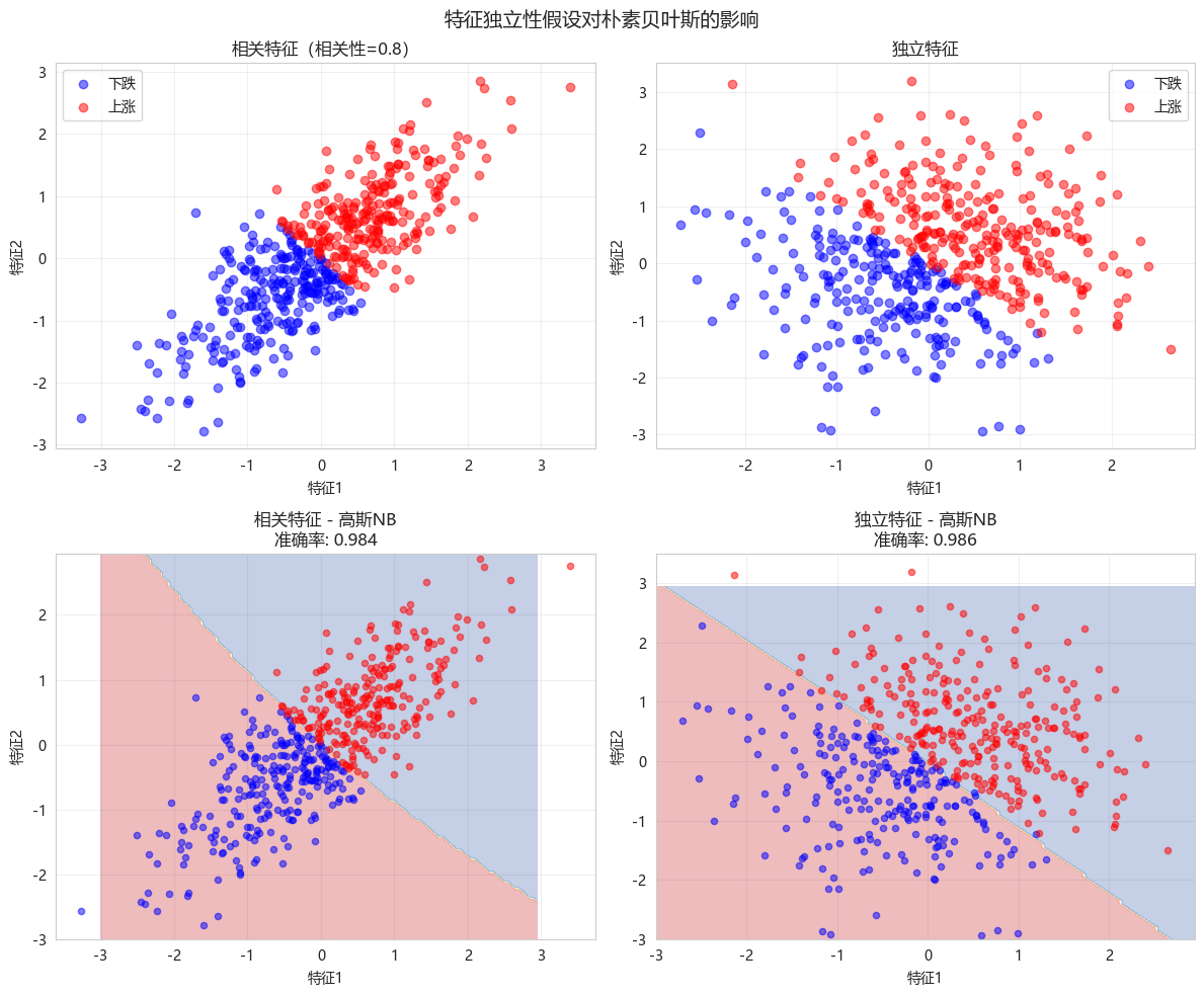
观察结论:
- 相关特征:决策边界仍合理,但概率估计有偏差
- 独立特征:朴素贝叶斯表现最佳
np.random.multivariate_normal用于生成多元高斯分布(多维正态分布)随机样本
pythonnp.random.multivariate_normal(mean, cov, size=None, check_valid='warn', tol=1e-8)参数说明:
- mean: 均值向量(长度为特征数)
- cov: 协方差矩阵(方阵,大小=特征数×特征数)
- size: 样本数量(整数或元组)
- check_valid: 矩阵有效性检查
- tol: 数值容差
3. 生成金融数据
python
def generate_financial_data(ts_code):
    """生成金融数据"""

    data_path = Path(r"E:\AppData\quant_trade\klines\kline2014-2024")
    kline_file = data_path / f"{ts_code}.csv"

    df = pd.read_csv(kline_file, usecols=["trade_date", "close", "vol"],
                     parse_dates=["trade_date"])\
            .rename(columns={"vol": "volume"})\
            .sort_values(by=["trade_date"])\
            .reset_index(drop=True)

    df['return'] = df['close'].pct_change()

    # 技术指标
    # RSI
    delta = df['return'].fillna(0)
    gain = delta.where(delta > 0, 0).rolling(14).mean()
    loss = -delta.where(delta < 0, 0).rolling(14).mean()
    rs = gain / (loss + 1e-10)
    df['rsi'] = 100 - (100 / (1 + rs))

    # MACD
    ema12 = df['close'].ewm(span=12, adjust=False).mean()
    ema26 = df['close'].ewm(span=26, adjust=False).mean()
    df['macd'] = ema12 - ema26
    df['macd_signal'] = df['macd'].ewm(span=9, adjust=False).mean()

    # 均线比率
    df['ma5'] = df['close'].rolling(5).mean()
    df['ma20'] = df['close'].rolling(20).mean()
    df['ma_ratio'] = df['ma5'] / df['ma20'] - 1

    # 波动率
    df['volatility'] = df['return'].rolling(20).std()

    # 成交量比率
    df['volume_ratio'] = df['volume'] / df['volume'].rolling(10).mean()

    # 动量指标
    for lag in [1, 2, 3, 5, 10]:
        df[f'momentum_{lag}'] = df['return'].shift(lag).fillna(0)

     # 目标变量:次日收益率
    df['future_return'] = df['return'].shift(-1)

    # 删除缺失值
    df = df.dropna()

    return df

# 生成数据
ts_code = "300033.SZ"
df = generate_financial_data(ts_code)
print(f"数据形状: {df.shape}")

# 特征选择
feature_cols = ['rsi', 'macd', 'macd_signal', 'ma_ratio', 'volatility',
                'volume_ratio', 'momentum_1', 'momentum_2', 'momentum_3',
                'momentum_5', 'momentum_10']
X = df[feature_cols].values
y_continuous = df['future_return'].values

print(f"特征数量: {len(feature_cols)}")
print(f"样本数量: {len(X)}")

# 按时间划分
split_idx = int(len(X) * 0.7)
X_train = X[:split_idx]
X_test = X[split_idx:]
y_train_cont = y_continuous[:split_idx]
y_test_cont = y_continuous[split_idx:]

print(f"\n训练集: {len(X_train)} 样本")
print(f"测试集: {len(X_test)} 样本")

# 数据标准化
scaler = StandardScaler()
X_train_scaled = scaler.fit_transform(X_train)
X_test_scaled = scaler.transform(X_test)数据形状: (2450, 18)
特征数量: 11
样本数量: 2450
训练集: 1715 样本
测试集: 735 样本4. 核心实战:极端涨跌预警模型(5档分类)
4.1 将连续收益率离散化为5档
python
def discretize_returns(returns, quantiles=[0.05, 0.2, 0.8, 0.95]):
    """
    将连续收益率离散化为5档
    档位: 0=大跌, 1=小跌, 2=平稳, 3=小涨, 4=大涨
    """
    thresholds = np.quantile(returns, quantiles)

    y_discrete = np.zeros(len(returns), dtype=int)
    y_discrete[returns <= thresholds[0]] = 0      # 大跌 (< 5%)
    y_discrete[(returns > thresholds[0]) & (returns <= thresholds[1])] = 1   # 小跌
    y_discrete[(returns > thresholds[1]) & (returns <= thresholds[2])] = 2   # 平稳
    y_discrete[(returns > thresholds[2]) & (returns <= thresholds[3])] = 3   # 小涨
    y_discrete[returns > thresholds[3]] = 4       # 大涨 (> 95%)

    return y_discrete, thresholds

# 使用训练集的分位数进行离散化
y_train_discrete, thresholds = discretize_returns(y_train_cont)
y_test_discrete = np.zeros(len(y_test_cont), dtype=int)
y_test_discrete[y_test_cont <= thresholds[0]] = 0
y_test_discrete[(y_test_cont > thresholds[0]) & (y_test_cont <= thresholds[1])] = 1
y_test_discrete[(y_test_cont > thresholds[1]) & (y_test_cont <= thresholds[2])] = 2
y_test_discrete[(y_test_cont > thresholds[2]) & (y_test_cont <= thresholds[3])] = 3
y_test_discrete[y_test_cont > thresholds[3]] = 4

# 显示档位分布
class_names = ['大跌', '小跌', '平稳', '小涨', '大涨']

print("="*60)
print("5档分类分布")
print("="*60)
print(f"\n分位数阈值: {thresholds}")
print("\n训练集分布:")
for i, name in enumerate(class_names):
    count = np.sum(y_train_discrete == i)
    print(f"  {name}: {count} ({count/len(y_train_discrete):.1%})")

print("\n测试集分布:")
for i, name in enumerate(class_names):
    count = np.sum(y_test_discrete == i)
    print(f"  {name}: {count} ({count/len(y_test_discrete):.1%})")

# 可视化分布
fig, axes = plt.subplots(1, 2, figsize=(12, 5))

axes[0].hist(y_train_cont, bins=50, edgecolor='black', alpha=0.7)
axes[0].axvline(x=thresholds[0], color='r', linestyle='--', label='5%分位')
axes[0].axvline(x=thresholds[1], color='orange', linestyle='--', label='20%分位')
axes[0].axvline(x=thresholds[2], color='green', linestyle='--', label='80%分位')
axes[0].axvline(x=thresholds[3], color='purple', linestyle='--', label='95%分位')
axes[0].set_xlabel('未来收益率')
axes[0].set_ylabel('频数')
axes[0].set_title('收益率分布与分位数')
axes[0].legend()
axes[0].grid(True, alpha=0.3)

axes[1].bar(class_names, [np.sum(y_train_discrete == i) for i in range(5)])
axes[1].set_xlabel('档位')
axes[1].set_ylabel('样本数')
axes[1].set_title('5档分类分布')
for i, count in enumerate([np.sum(y_train_discrete == i) for i in range(5)]):
    axes[1].text(i, count + 5, str(count), ha='center')

plt.tight_layout()
plt.show()============================================================
5档分类分布
============================================================
分位数阈值: [-0.0603375 -0.02166747 0.02484053 0.09525333]
训练集分布:
大跌: 86 (5.0%)
小跌: 257 (15.0%)
平稳: 1029 (60.0%)
小涨: 257 (15.0%)
大涨: 86 (5.0%)
测试集分布:
大跌: 14 (1.9%)
小跌: 118 (16.1%)
平稳: 489 (66.5%)
小涨: 101 (13.7%)
大涨: 13 (1.8%)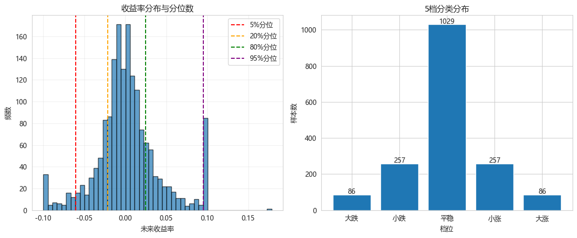
np.quantile用于计算分位数(Quantile)
pythonnp.quantile(a, q, axis=None, out=None, overwrite_input=False, method='linear', keepdims=False)主要参数:
- a: 输入数组
- q: 要计算的分位数(0-1之间的数值或数组)
- axis: 沿哪个轴计算(None表示全部元素)
- method: 插值方法
- keepdims: 是否保持维度
4.2 高斯朴素贝叶斯(5档分类)
python
print("="*60)
print("高斯朴素贝叶斯 - 5档分类")
print("="*60)

gnb = GaussianNB()
gnb.fit(X_train_scaled, y_train_discrete)

# 预测
y_pred_gnb = gnb.predict(X_test_scaled)
y_proba_gnb = gnb.predict_proba(X_test_scaled)

# 评估
acc = accuracy_score(y_test_discrete, y_pred_gnb)
print(f"准确率: {acc:.4f}")

# 分类报告
print("\n分类报告:")
print(classification_report(y_test_discrete, y_pred_gnb,
                           target_names=class_names))

# 混淆矩阵
cm = confusion_matrix(y_test_discrete, y_pred_gnb)
plt.figure(figsize=(10, 8))
sns.heatmap(cm, annot=True, fmt='d', cmap='Blues',
            xticklabels=class_names, yticklabels=class_names)
plt.xlabel('预测')
plt.ylabel('真实')
plt.title('高斯朴素贝叶斯 - 混淆矩阵')
plt.show()============================================================
高斯朴素贝叶斯 - 5档分类
============================================================
准确率: 0.6082
分类报告:
precision recall f1-score support
大跌 0.08 0.14 0.10 14
小跌 0.32 0.14 0.20 118
平稳 0.71 0.87 0.78 489
小涨 0.06 0.02 0.03 101
大涨 0.12 0.23 0.15 13
accuracy 0.61 735
macro avg 0.26 0.28 0.25 735
weighted avg 0.54 0.61 0.56 735
4.3 极端涨跌预警性能分析
python
def analyze_extreme_predictions(y_true, y_pred, class_names):
    """分析极端涨跌(大跌/大涨)的预测性能"""

    # 极端涨跌的类别索引
    extreme_classes = {'大跌': 0, '大涨': 4}

    print("="*60)
    print("极端涨跌预警性能分析")
    print("="*60)

    for name, class_idx in extreme_classes.items():
        # 二分类:是否为该极端情况
        y_true_binary = (y_true == class_idx).astype(int)
        y_pred_binary = (y_pred == class_idx).astype(int)

        # 计算指标
        precision = precision_score(y_true_binary, y_pred_binary, zero_division=0)
        recall = recall_score(y_true_binary, y_pred_binary, zero_division=0)
        f1 = f1_score(y_true_binary, y_pred_binary, zero_division=0)

        # 混淆矩阵
        tn, fp, fn, tp = confusion_matrix(y_true_binary, y_pred_binary).ravel()

        print(f"\n{name} 预警性能:")
        print(f"  精确率: {precision:.4f} (预测为{name}中实际为{name}的比例)")
        print(f"  召回率: {recall:.4f} (实际{name}中被正确识别的比例)")
        print(f"  F1分数: {f1:.4f}")
        print(f"  正确预警次数: {tp}")
        print(f"  误报次数: {fp}")
        print(f"  漏报次数: {fn}")

analyze_extreme_predictions(y_test_discrete, y_pred_gnb, class_names)============================================================
极端涨跌预警性能分析
============================================================
大跌 预警性能:
精确率: 0.0769 (预测为大跌中实际为大跌的比例)
召回率: 0.1429 (实际大跌中被正确识别的比例)
F1分数: 0.1000
正确预警次数: 2
误报次数: 24
漏报次数: 12
大涨 预警性能:
精确率: 0.1154 (预测为大涨中实际为大涨的比例)
召回率: 0.2308 (实际大涨中被正确识别的比例)
F1分数: 0.1538
正确预警次数: 3
误报次数: 23
漏报次数: 104.4 不同阈值下的极端预警效果
python
def analyze_threshold_impact(y_true_proba, y_true_class, extreme_class_idx=4):
    """分析不同概率阈值下的极端预警效果"""

    thresholds = np.arange(0.1, 0.9, 0.05)
    precisions = []
    recalls = []

    for thresh in thresholds:
        y_pred_binary = (y_true_proba[:, extreme_class_idx] >= thresh).astype(int)
        y_true_binary = (y_true_class == extreme_class_idx).astype(int)

        precisions.append(precision_score(y_true_binary, y_pred_binary, zero_division=0))
        recalls.append(recall_score(y_true_binary, y_pred_binary, zero_division=0))

    plt.figure(figsize=(10, 6))
    plt.plot(thresholds, precisions, 'b-o', label='精确率', linewidth=2)
    plt.plot(thresholds, recalls, 'r-s', label='召回率', linewidth=2)
    plt.xlabel('概率阈值')
    plt.ylabel('分数')
    plt.title('高斯NB - "大涨"预警阈值影响分析')
    plt.legend()
    plt.grid(True, alpha=0.3)

    # 找到最佳F1阈值
    f1_scores = 2 * np.array(precisions) * np.array(recalls) / (np.array(precisions) + np.array(recalls) + 1e-10)
    best_idx = np.argmax(f1_scores)
    plt.axvline(x=thresholds[best_idx], color='g', linestyle='--',
                label=f'最佳阈值={thresholds[best_idx]:.2f} (F1={f1_scores[best_idx]:.3f})')
    plt.legend()
    plt.show()

analyze_threshold_impact(y_proba_gnb, y_test_discrete, extreme_class_idx=4)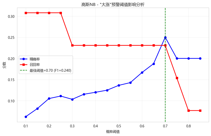
5. 三种朴素贝叶斯模型对比
5.1 数据准备(二值化和多项式格式)
python
# 伯努利NB需要二值特征
binarizer = KBinsDiscretizer(n_bins=5, encode='ordinal', strategy='quantile')
X_train_binned = binarizer.fit_transform(X_train_scaled)
X_test_binned = binarizer.transform(X_test_scaled)

# 多项式NB需要非负整数特征(转换为0-4)
X_train_multinomial = X_train_binned.astype(int)
X_test_multinomial = X_test_binned.astype(int)

# 伯努利NB需要二值特征(0/1)
X_train_bernoulli = (X_train_scaled > 0).astype(int)
X_test_bernoulli = (X_test_scaled > 0).astype(int)
5.2 模型训练与对比
python
plt.rcParams['axes.unicode_minus'] = False

def compare_naive_bayes_models(X_train_dict, X_test_dict, y_train, y_test, class_names):
    """对比三种朴素贝叶斯模型"""

    models = {
        '高斯NB': GaussianNB(),
        '多项式NB': MultinomialNB(alpha=1.0),
        '伯努利NB': BernoulliNB(alpha=1.0)
    }

    results = []
    predictions = {}

    print("="*70)
    print("三种朴素贝叶斯模型对比")
    print("="*70)
    print(f"\n{'模型':<12} {'准确率':<10} {'精确率(宏平均)':<15} {'召回率(宏平均)':<15} {'F1(宏平均)':<12}")
    print("-"*70)

    for name, model in models.items():
        # 选择对应的数据
        if name == '高斯NB':
            X_train = X_train_dict['gaussian']
            X_test = X_test_dict['gaussian']
        elif name == '多项式NB':
            X_train = X_train_dict['multinomial']
            X_test = X_test_dict['multinomial']
        else:
            X_train = X_train_dict['bernoulli']
            X_test = X_test_dict['bernoulli']

        start_time = time.time()
        model.fit(X_train, y_train)
        train_time = time.time() - start_time

        start_time = time.time()
        y_pred = model.predict(X_test)
        predict_time = time.time() - start_time

        acc = accuracy_score(y_test, y_pred)
        prec_macro = precision_score(y_test, y_pred, average='macro', zero_division=0)
        rec_macro = recall_score(y_test, y_pred, average='macro', zero_division=0)
        f1_macro = f1_score(y_test, y_pred, average='macro', zero_division=0)

        results.append({
            'model': name,
            'accuracy': acc,
            'precision_macro': prec_macro,
            'recall_macro': rec_macro,
            'f1_macro': f1_macro,
            'train_time': train_time,
            'predict_time': predict_time
        })

        predictions[name] = y_pred

        print(f"{name:<12} {acc:<10.4f} {prec_macro:<15.4f} {rec_macro:<15.4f} {f1_macro:<12.4f}")

    results_df = pd.DataFrame(results)

    # 可视化对比
    fig, axes = plt.subplots(1, 2, figsize=(14, 5))

    metrics = ['accuracy', 'precision_macro', 'recall_macro', 'f1_macro']
    x = np.arange(len(models))
    width = 0.2

    for i, metric in enumerate(metrics):
        axes[0].bar(x + i*width, results_df[metric], width, label=metric)
    axes[0].set_xticks(x + width*1.5)
    axes[0].set_xticklabels(results_df['model'])
    axes[0].set_ylabel('分数')
    axes[0].set_title('模型性能对比')
    axes[0].legend()
    axes[0].grid(True, alpha=0.3)

    # 时间对比
    axes[1].bar(x - width/2, results_df['train_time'], width, label='训练时间', color='blue')
    axes[1].bar(x + width/2, results_df['predict_time'], width, label='预测时间', color='red')
    axes[1].set_xticks(x)
    axes[1].set_xticklabels(results_df['model'])
    axes[1].set_ylabel('时间 (秒)')
    axes[1].set_title('训练与预测时间对比')
    axes[1].legend()
    axes[1].set_yscale('log')
    axes[1].grid(True, alpha=0.3)

    plt.suptitle('三种朴素贝叶斯模型综合对比', fontsize=14)
    plt.tight_layout()
    plt.show()

    return results_df, predictions

# 准备数据字典
X_train_dict = {
    'gaussian': X_train_scaled,
    'multinomial': X_train_multinomial,
    'bernoulli': X_train_bernoulli
}
X_test_dict = {
    'gaussian': X_test_scaled,
    'multinomial': X_test_multinomial,
    'bernoulli': X_test_bernoulli
}

results_df, predictions = compare_naive_bayes_models(
    X_train_dict, X_test_dict,
    y_train_discrete, y_test_discrete,
    class_names
)======================================================================
三种朴素贝叶斯模型对比
======================================================================
模型 准确率 精确率(宏平均) 召回率(宏平均) F1(宏平均)
----------------------------------------------------------------------
高斯NB 0.6082 0.2563 0.2805 0.2524
多项式NB 0.6639 0.2670 0.2024 0.1669
伯努利NB 0.6340 0.2501 0.2495 0.2104 
5.3 各模型针对极端涨跌的预警效果
python
def compare_extreme_detection(predictions_dict, y_true, class_names):
    """对比各模型对极端涨跌的检测能力"""

    extreme_classes = {'大跌': 0, '大涨': 4}

    fig, axes = plt.subplots(1, 2, figsize=(12, 5))

    for idx, (extreme_name, class_idx) in enumerate(extreme_classes.items()):
        y_true_binary = (y_true == class_idx).astype(int)

        precisions = []
        recalls = []
        model_names = []

        for model_name, y_pred in predictions_dict.items():
            y_pred_binary = (y_pred == class_idx).astype(int)
            precisions.append(precision_score(y_true_binary, y_pred_binary, zero_division=0))
            recalls.append(recall_score(y_true_binary, y_pred_binary, zero_division=0))
            model_names.append(model_name)

        x = np.arange(len(model_names))
        width = 0.35

        axes[idx].bar(x - width/2, precisions, width, label='精确率', color='blue')
        axes[idx].bar(x + width/2, recalls, width, label='召回率', color='red')
        axes[idx].set_xticks(x)
        axes[idx].set_xticklabels(model_names)
        axes[idx].set_ylabel('分数')
        axes[idx].set_title(f'{extreme_name} 预警性能')
        axes[idx].legend()
        axes[idx].grid(True, alpha=0.3)
        axes[idx].set_ylim(0, 1)

    plt.suptitle('各模型极端涨跌预警性能对比', fontsize=14)
    plt.tight_layout()
    plt.show()

compare_extreme_detection(predictions, y_test_discrete, class_names)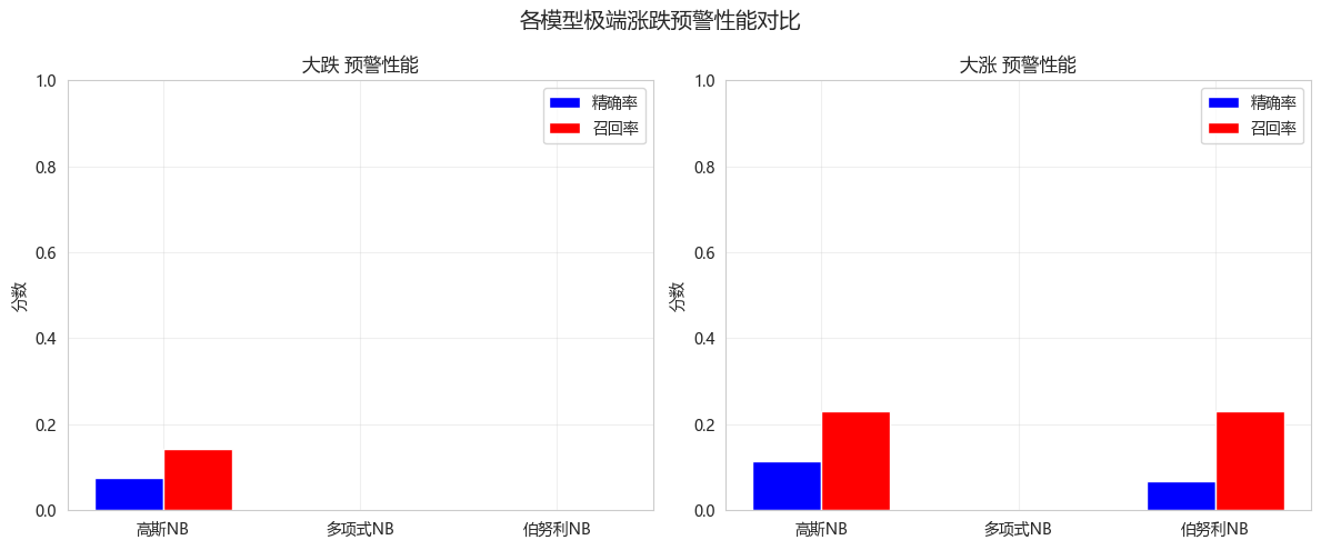
5.4 拉普拉斯平滑效果演示
python
def demonstrate_laplace_smoothing():
    """演示拉普拉斯平滑的效果"""
    from sklearn.naive_bayes import MultinomialNB

    # 创建稀疏数据(很多0)
    np.random.seed(42)
    X_sparse = np.random.choice([0, 1], size=(500, 20), p=[0.8, 0.2])
    y_sparse = np.random.choice([0, 1], size=500)

    alpha_values = [0, 0.1, 0.5, 1.0, 2.0, 5.0]
    scores = []

    for alpha in alpha_values:
        mnb = MultinomialNB(alpha=alpha)
        cv_scores = cross_val_score(mnb, X_sparse, y_sparse, cv=5)
        scores.append(cv_scores.mean())

    plt.figure(figsize=(10, 6))
    plt.plot(alpha_values, scores, 'bo-', linewidth=2, markersize=8)
    plt.xlabel('alpha (平滑参数)')
    plt.ylabel('交叉验证准确率')
    plt.title('拉普拉斯平滑参数对稀疏数据的影响')
    plt.grid(True, alpha=0.3)

    # 标记最佳alpha
    best_idx = np.argmax(scores)
    plt.axvline(x=alpha_values[best_idx], color='r', linestyle='--',
                label=f'最佳 alpha={alpha_values[best_idx]}')
    plt.legend()
    plt.show()

    print("观察结论:")
    print("- alpha=0 (无平滑): 可能因零概率导致性能差")
    print("- alpha=1 (加一平滑): 常用默认值")
    print("- 过大的alpha: 过度平滑,性能下降")

demonstrate_laplace_smoothing()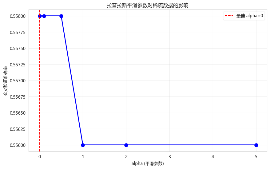
观察结论:
- alpha=0 (无平滑): 可能因零概率导致性能差
- alpha=1 (加一平滑): 常用默认值
- 过大的alpha: 过度平滑,性能下降
6. 特征重要性分析
高斯NB的特征分布
python
def analyze_gnb_feature_distributions(model, feature_names, class_names):
    """分析高斯NB中每个类别下特征的均值"""

    means = model.theta_  # 每个类别的特征均值
    variances = model.var_  # 每个类别的特征方差

    fig, axes = plt.subplots(2, 3, figsize=(15, 10))
    axes = axes.ravel()

    # 选择几个关键特征
    selected_features = [0, 1, 2, 3, 4, 5]

    for idx, f_idx in enumerate(selected_features):
        if idx >= len(axes):
            break

        bar_color_map = {
            '大涨': 'red',
            '小涨': 'gray',
            '平稳': 'gray',
            '小跌': 'gray',
            '大跌': 'green',
        }

        for c in range(len(class_names)):
            axes[idx].bar(c, means[c, f_idx], color=bar_color_map[class_names[c]],
                         alpha=0.7, label=class_names[c] if idx == 0 else "")

        axes[idx].set_xticks(range(len(class_names)))
        axes[idx].set_xticklabels(class_names, rotation=45)
        axes[idx].set_title(f'特征: {feature_names[f_idx]}')
        axes[idx].set_ylabel('均值')
        axes[idx].grid(True, alpha=0.3)

    axes[0].legend()
    plt.suptitle('高斯朴素贝叶斯 - 各类别下的特征均值分布', fontsize=14)
    plt.tight_layout()
    plt.show()

analyze_gnb_feature_distributions(gnb, feature_cols, class_names)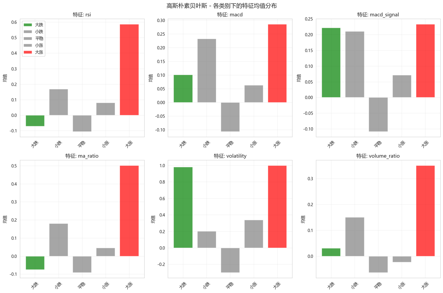
7. 朴素贝叶斯 vs 其他模型
python
# 对比朴素贝叶斯与随机森林、逻辑回归
from sklearn.linear_model import LogisticRegression
from sklearn.ensemble import RandomForestClassifier

print("="*60)
print("朴素贝叶斯 vs 其他模型对比")
print("="*60)

# 逻辑回归(多分类)
lr = LogisticRegression(max_iter=1000, multi_class='ovr', random_state=42)
lr.fit(X_train_scaled, y_train_discrete)
lr_pred = lr.predict(X_test_scaled)

# 随机森林
rf = RandomForestClassifier(n_estimators=100, max_depth=10, random_state=42)
rf.fit(X_train_scaled, y_train_discrete)
rf_pred = rf.predict(X_test_scaled)

# 对比结果
models_compare = {
    '高斯NB': y_pred_gnb,
    '逻辑回归': lr_pred,
    '随机森林': rf_pred
}

print(f"\n{'模型':<12} {'准确率':<10} {'精确率(宏平均)':<15} {'召回率(宏平均)':<15} {'F1(宏平均)':<12}")
print("-"*70)

for name, y_pred in models_compare.items():
    acc = accuracy_score(y_test_discrete, y_pred)
    prec = precision_score(y_test_discrete, y_pred, average='macro', zero_division=0)
    rec = recall_score(y_test_discrete, y_pred, average='macro', zero_division=0)
    f1 = f1_score(y_test_discrete, y_pred, average='macro', zero_division=0)
print(f"{name:<12} {acc:<10.4f} {prec:<15.4f} {rec:<15.4f} {f1:<12.4f}")============================================================
朴素贝叶斯 vs 其他模型对比
============================================================
模型 准确率 精确率(宏平均) 召回率(宏平均) F1(宏平均)
----------------------------------------------------------------------
高斯NB 0.6082 0.2563 0.2805 0.2524
逻辑回归 0.6612 0.2304 0.2317 0.2088
随机森林 0.6517 0.2120 0.2052 0.1798 8. 今日总结
-
朴素贝叶斯核心原理:
- 基于贝叶斯定理:P(y|x) ∝ P(x|y)·P(y)
- 特征条件独立假设(朴素假设)
- 生成式模型,训练极快
-
三种模型:
- 高斯NB:连续特征,假设正态分布
- 多项式NB:离散计数,如词频
- 伯努利NB:二值特征,如布尔值
-
极端涨跌预警应用:
- 将收益率离散化为5档(大跌/小跌/平稳/小涨/大涨)
- 高斯NB快速分类,识别极端情况
- 可以调整概率阈值平衡精确率和召回率
-
拉普拉斯平滑:
- 解决零概率问题
- alpha=1 是常用默认值
-
优缺点:
- 优点:极快、小数据友好、可解释
- 缺点:独立假设、概率估计不准
-
扩展作业
- 作业1:尝试不同的分箱策略(等频、等宽),对比效果
- 作业2:实现自定义的朴素贝叶斯(不同的分布假设)
- 作业3:使用朴素贝叶斯作为实时风控预警系统的一部分
- 作业4:对比平滑参数alpha对模型性能的影响
-
量化思考
- 朴素贝叶斯非常适合作为快速预警系统
- 在真实交易中,可以作为第一道筛选器
- 极端涨跌预测的召回率比精确率更重要
- 可结合其他模型形成多级预警体系