目录
[1.Apollo MPC Controller架构](#1.Apollo MPC Controller架构)
Apollo MPC Controller中同时对横纵向控制进行求解,而本文只针对横向控制进行求解,其中会使用到OSQP求解器对MPC问题求解。
1.Apollo MPC Controller架构
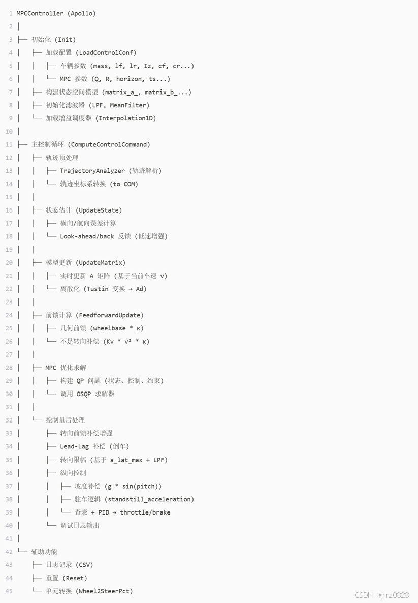
下图为Apollo MPC Controller架构,本文主要关注MPC优化求解这一部分。
│ ├── MPC 优化求解
│ │ ├── 构建 QP 问题 (状态、控制、约束)
│ │ └── 调用 OSQP 求解器
2.Mpc_Osqp类
2.1Mpc_Osqp类成员函数
|-------------------------------|-----------------------------------------------------|
| 成员函数 | 作用 |
| MpcOsqp() | 构造函数 |
| Solve() | 针对MPC问题调用OSQP求解器求解 |
| CalculateKernel() | 构建 Hessian 矩阵 P (对应代价函数的二次项) |
| CalculateEqualityConstraint() | 构建等式约束(系统动态)和不等式约束(边界)的矩阵 A (OSQP 中统一处理为不等式 l≤Ax≤u) |
| CalculateGradient() | 计算线性项 q (即 gradient_),通常来自参考轨迹和代价矩阵 |
| CalculateConstraintVectors() | 构建约束上下界向量 lowerBound_ 和 upperBound_,对应 OSQP 的 l和u |
| Settings() | OSQP 的配置(如最大迭代、精度) |
| Data() | OSQP 的问题数据(P, q, A, l, u) |
| FreeData() | 释放 OSQP 数据结构的内存 |
| CopyData() | 将 std::vector 转换为 C 风格数组 |
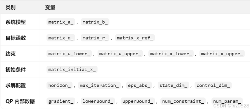
2.2Mpc_Osqp类成员变量
|-------------------|-----------------------------------------------------------------|-------------------|
| 成员函数 | 维度 | 作用 |
| matrix_a_ | state_dim_ × state_dim_ | 状态矩阵A离散化 |
| matrix_b_ | state_dim_ × control_dim_ | 控制矩阵B离散化 |
| matrix_q_ | state_dim_ × state_dim_ | 状态权重矩阵Q |
| matrix_r_ | control_dim_ × control_dim_ | 控制权重矩阵R |
| matrix_initial_x_ | state_dim_ × 1 | 当前状态量 |
| matrix_u_lower_ | control_dim_ × horizon_ | 控制量下界 |
| matrix_u_upper_ | control_dim_ × horizon_ | 控制量上界 |
| matrix_x_lower_ | state_dim_ × (horizon_ + 1) | 状态量下界 |
| matrix_x_upper_ | state_dim_ × (horizon_ + 1) | 状态量上界 |
| matrix_x_ref_ | state_dim_ × (horizon_ + 1) | 参考状态量 |
| max_iteration_ | | 最大迭代次数 |
| horizon_ | | 预测步长 |
| eps_abs_ | | 求解精度 |
| state_dim_ | | 状态量维度 |
| control_dim_ | | 控制量维度 |
| num_param_ | state_dim_ * (N + 1) + control_dim_ * N | 总优化变量数 |
| num_constraint_ | state_dim_ * N(等式) + (control_dim_ + state_dim_) * N(不等式,若启用) | 总约束数量= 等式约束+不等式约束 |
| gradient_ | 同num_param_ | QP 目标函数线性项q |
| lowerBound_ | 同num_constraint_ | 所有约束的下界向量l |
| upperBound_ | 同num_constraint_ | 所有约束的上界向量u |
2.3Mpc_Osqp初始化
cpp
MpcOsqp::MpcOsqp(const Eigen::MatrixXd &matrix_a,
                 const Eigen::MatrixXd &matrix_b,
                 const Eigen::MatrixXd &matrix_q,
                 const Eigen::MatrixXd &matrix_r,
                 const Eigen::MatrixXd &matrix_initial_x,
                 const Eigen::MatrixXd &matrix_u_lower,
                 const Eigen::MatrixXd &matrix_u_upper,
                 const Eigen::MatrixXd &matrix_x_lower,
                 const Eigen::MatrixXd &matrix_x_upper,
                 const Eigen::MatrixXd &matrix_x_ref, const int max_iter,
                 const int horizon, const double eps_abs)
    : matrix_a_(matrix_a),
      matrix_b_(matrix_b),
      matrix_q_(matrix_q),
      matrix_r_(matrix_r),
      matrix_initial_x_(matrix_initial_x),
      matrix_u_lower_(matrix_u_lower),
      matrix_u_upper_(matrix_u_upper),
      matrix_x_lower_(matrix_x_lower),
      matrix_x_upper_(matrix_x_upper),
      matrix_x_ref_(matrix_x_ref),
      max_iteration_(max_iter),
      horizon_(horizon),
      eps_abs_(eps_abs) {
  state_dim_ = matrix_b.rows();
  control_dim_ = matrix_b.cols();
  ADEBUG << "state_dim" << state_dim_;
  ADEBUG << "control_dim_" << control_dim_;
  num_param_ = state_dim_ * (horizon_ + 1) + control_dim_ * horizon_;
}
|--------------------|----------------------------------|
| 参数 | 含义 |
| matrix_ad_ | 状态矩阵A离散化 |
| matrix_bd_ | 控制矩阵B离散化 |
| matrix_q_updated_ | 状态权重矩阵 |
| matrix_r_updated_ | 控制权重矩阵 |
| matrix_state_ | 当前状态量ed,dot_ed,efai,dot_efai |
| lower_bound | 控制量下界 |
| upper_bound | 控制量上界 |
| lower_state_bound | 状态量下界 |
| upper_state_bound | 状态量上界 |
| reference_state | 参考状态量 |
| mpc_max_iteration_ | 最大迭代次数 |
| horizon_ | 预测步长 |
| mpc_eps_ | 求解精度 |
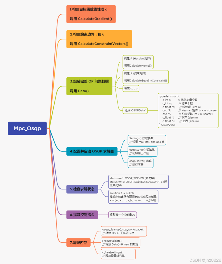
2.4Mpc_Osqp类的执行顺序
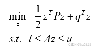
3.MPC问题相关矩阵的构造
将MPC问题转换为如下二次规划形式:
3.1优化变量z
优化变量从u变为z,维度增加,但是矩阵变得稀疏之后求解速度可以变得更快,还能对控制变量和状态变量进行约束。
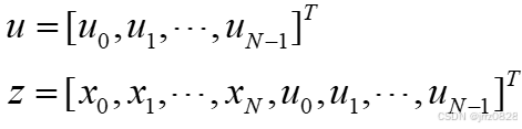
Apollo 中将状态量x和控制量u一起作为优化变量z,是为了将 MPC 问题转化为一个具有高度稀疏结构的 QP 问题,从而能被 OSQP 等求解器高效、实时地求解。虽然变量数量增加了,但稀疏性带来的计算效率提升远远超过变量增加的开销,这是现代 MPC 实现(尤其在自动驾驶、机器人领域)的标准做法。
本质是:用更多变量 + 更多约束,换取矩阵的稀疏性,从而获得更快的求解速度
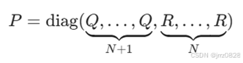
3.2P矩阵的构造
P矩阵是horizon+1个Q矩阵和horizon个R矩阵组合而成的对角矩阵,需要将其转换为CSC格式。
|-----------|-------------------------------------------------------------------------------|
| 数组 | 含义 |
| P_data | 所有非零元素的值,按列优先(column-major)顺序存储 |
| P_indices | 每个非零元素对应的行号 |
| P_indptr | 长度为 n + 1 的数组,col_ptrj 表示第 j 列的第一个非零元在 P_data中的索引; col_ptrn = 总非零元个数。 |
例如P矩阵为
1 0 0 0
2 5 0 0
3 0 6 0
4 0 7 8
P_data:1, 2, 3, 4, 5, 6, 7, 8
P_indices:0, 1, 2, 3, 1, 2, 3, 3
P_indptr:0, 4, 5, 7, 8
3.3q矩阵的构造
实际上作为参考值,在Apollo中都设置为0了。
cpp
Eigen::MatrixXd reference_state = Eigen::MatrixXd::Zero(basic_state_size_, 1);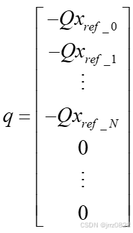
3.4A矩阵的构造
等式约束也统一写成不等式约束:
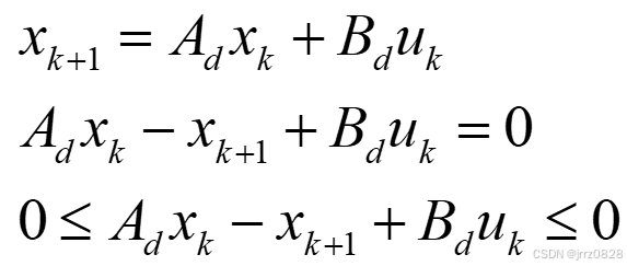
所有约束如下所示:
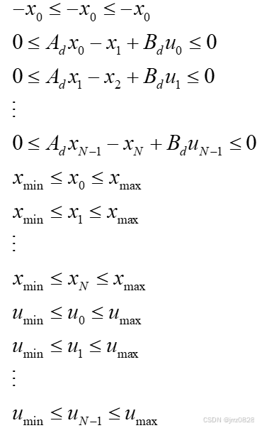
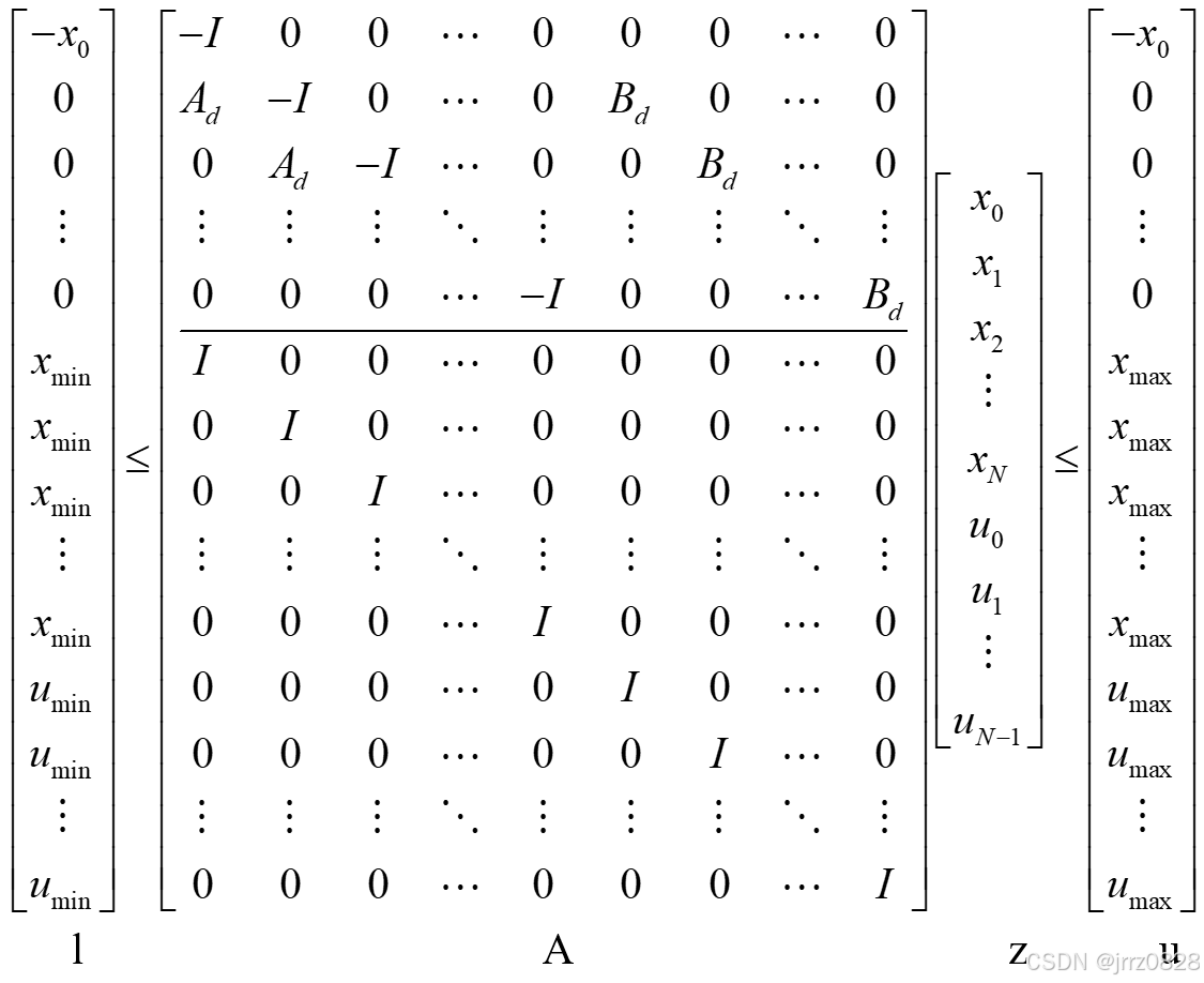
写成矩阵形式,可以得到A、l 、u矩阵的构造:
3.5l和u的构造
见3.4节。
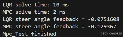
4.MPC问题求解的实时性
对比LQR和MPC求解所用的时间,其中LQR中Riccati方程的求解采用的是迭代法。
4.1SolveLQRProblem
cpp
void Mpc_Test::SolveLQRProblem() {
	Eigen::MatrixXd &A = matrixAd_;
	Eigen::MatrixXd &B = matrixBd_;
	Eigen::MatrixXd &Q = matrixQ_updated_;
	Eigen::MatrixXd &R = matrixR_;

	double tolerance = eps_;
	int max_num_iteration = max_iteration_;
	Eigen::MatrixXd *ptr_K = &matrixK_;

	if (A.rows() != A.cols() || B.rows() != A.rows() || Q.rows() != Q.cols()
			|| Q.rows() != A.rows() || R.rows() != R.cols()
			|| R.rows() != B.cols()) {
		return;
	}

	Eigen::MatrixXd AT = A.transpose();
	Eigen::MatrixXd BT = B.transpose();

// Solves a discrete-time Algebraic Riccati equation (DARE)
// Calculate Matrix Difference Riccati Equation, initialize P and Q
	Eigen::MatrixXd P = Q;
	int num_iteration = 0;
	float diff = std::numeric_limits<float>::max();
	Eigen::MatrixXd P_next = P;
	Eigen::MatrixXd P_next_diff = P;

    auto start = std::chrono::steady_clock::now();
	if (riccati_equation_solve_method_ == 1) {
		// 解析法求解
		// P = DiscreteAlgebraicRiccatiEquation(A, B, Q, R);
	} else if (riccati_equation_solve_method_ == 2) {
		// 迭代法求解
		while (num_iteration++ < max_num_iteration && diff > tolerance) {
			P_next = AT * P * A
					- AT * P * B * (R + BT * P * B).inverse() * BT * P * A + Q;
			P_next_diff = P_next - P;
			diff = fabs(P_next_diff.maxCoeff());
			P = P_next;
		}
	}
	*ptr_K = (R + BT * P * B).inverse() * BT * P * A;
    auto end = std::chrono::steady_clock::now();
    auto ms = std::chrono::duration_cast<std::chrono::milliseconds>(end - start).count();

    std::cout << "LQR solve time: " << ms << " ms" << std::endl;
}
4.2SolveMPCProblem
cpp
void Mpc_Test::SolveMPCProblem() {
    auto start = std::chrono::steady_clock::now();
    // 存储osqp求解后的控制量
    Eigen::MatrixXd control_matrix = Eigen::MatrixXd::Zero(controls_, 1);
    std::vector<Eigen::MatrixXd> control(horizon_, control_matrix);

    // Eigen::MatrixXd control_gain_matrix = Eigen::MatrixXd::Zero(controls_, basic_state_size_);
    // std::vector<Eigen::MatrixXd> control_gain(horizon_, control_gain_matrix);

    // Eigen::MatrixXd addition_gain_matrix = Eigen::MatrixXd::Zero(controls_, 1);
    // std::vector<Eigen::MatrixXd> addition_gain(horizon_, addition_gain_matrix);

    // 构造相应的矩阵,用于MpcOsqp mpc_osqp初始化
    // lower_bound, upper_bound, lower_state_bound, upper_state_bound, reference_state,
    Eigen::MatrixXd reference_state = Eigen::MatrixXd::Zero(basic_state_size_, 1);
    std::vector<Eigen::MatrixXd> reference(horizon_, reference_state);

    Eigen::MatrixXd lower_bound(controls_, 1);
    lower_bound << -wheel_single_direction_max_degree_;

    Eigen::MatrixXd upper_bound(controls_, 1);
    upper_bound << wheel_single_direction_max_degree_;

    const double max = 1.0;
    Eigen::MatrixXd lower_state_bound(basic_state_size_, 1);
    Eigen::MatrixXd upper_state_bound(basic_state_size_, 1);

    // lateral_error, lateral_error_rate, heading_error, heading_error_rate
    // station_error, station_error_rate
    lower_state_bound << -1.0 * max, -1.0 * max, -1.0 * 3.1415926, -1.0 * max;
    upper_state_bound << max, max, 3.1415926, max;
    // mpc_osqp.Solve(&control_cmd)求解的结果
    std::vector<double> control_cmd(controls_, 0);
    // MpcOsqp mpc_osqp初始化
    MpcOsqp mpc_osqp(
        matrixAd_, matrixBd_, matrixQ_mpc_, matrixR_,
        matrixState_, lower_bound, upper_bound, lower_state_bound,
        upper_state_bound, reference_state, mpc_max_iteration_, horizon_,
        mpc_eps_);
    if (!mpc_osqp.Solve(&control_cmd)) {
        //std::cout << "MPC OSQP solver failed" << std::endl;
    } else {
        //std::cout << "MPC OSQP problem solved! " << std::endl;
        control[0](0, 0) = control_cmd.at(0);
        mpc_steer_angle_feedback_ = control[0](0, 0);
    }

    auto end = std::chrono::steady_clock::now();
    auto ms = std::chrono::duration_cast<std::chrono::milliseconds>(end - start).count();
    // 打印MPC问题的求解时间
    std::cout << "MPC solve time: " << ms << " ms" << std::endl;
}