Transformer 整体架构：一张图看懂

〇、为什么这一篇是分水岭

到这里，前 19 篇已经把 Transformer 的所有重要部件单独讲了一遍：

第 9--13 篇把 attention 拆开讲清了 Q、K、V、点积、softmax、scale 因子。
第 11 篇讲了位置编码------为什么 attention 需要它、sin/cos 是怎么设计的。
第 14 篇讲了 FFN 的角色------非线性、记忆容量、激活函数。
第 15 篇讲了残差与归一化------梯度的高速公路。
第 16 篇讲了 Multi-Head------多视角并行。
第 17 篇讲了 causal mask------自回归的工程基础。
第 18 篇讲了 <math xmlns="http://www.w3.org/1998/Math/MathML"> O ( n 2 ) O(n^2) </math>O(n2) 复杂度------长上下文的根本约束。
第 19 篇讲了原论文的历史背景------这一切是怎么诞生的。

但 19 篇的逐个零件讲解，到这里必须合成一张完整的图。只有当你能闭着眼睛说出「一个 token 从被 tokenize 那一刻起，到最终 softmax 出概率分布，中间经过了哪 N 步」时，你才算真正理解 Transformer。

这一篇就来做这件事。我不再讲新东西（新概念全在前 19 篇），而是把所有部件串起来，跟随一个具体的 token 走完它在 Transformer 里的旅程。读完后你应该能徒手画出 Transformer 的全貌、解释每一个箭头的存在理由、说出训练时和推理时数据流的差异。

原文链接

一、一张图：Transformer 的全貌

下图是论文 Figure 1 的清晰重绘版本，左边是 encoder（堆 <math xmlns="http://www.w3.org/1998/Math/MathML"> N = 6 N=6 </math>N=6 层），右边是 decoder（堆 <math xmlns="http://www.w3.org/1998/Math/MathML"> N = 6 N=6 </math>N=6 层），中间通过 cross-attention 连接：

这张重绘图在结构上与原论文 Figure 1 一致，只是为了教学可读性做了几处展开：把 positional encoding 与 embedding 合并显示、把 decoder 里的 encoder-decoder attention 直接标成了 cross-attention、把顶端输出头展开成了 linear <math xmlns="http://www.w3.org/1998/Math/MathML"> → \to </math>→ softmax <math xmlns="http://www.w3.org/1998/Math/MathML"> → \to </math>→ output probabilities。原图的本地副本见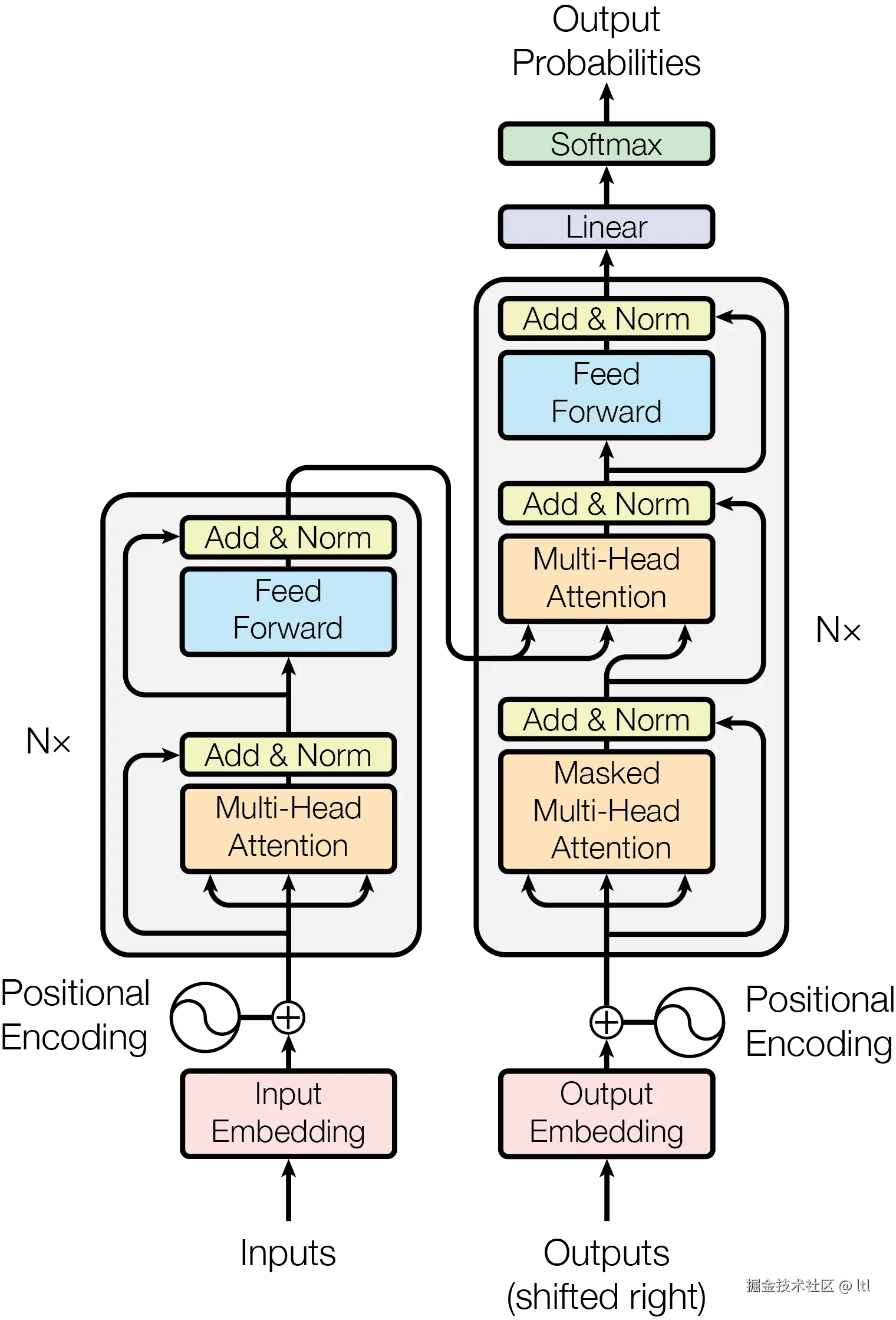，官方来源可对照 arXiv HTML 的 Figure 1，图片直链见 arXiv PNG，PDF 版可见 NeurIPS proceedings。arXiv HTML 页面注明：在署名条件下，Google 允许将论文中的 tables and figures 用于 journalistic or scholarly works 的转载。

把这张图刻进脑子里。它的关键骨架是：

左边 encoder：处理源语言（待翻译的句子）。
右边 decoder：生成目标语言（翻译输出）。
encoder 输出 → decoder 的 cross-attention：这是两边唯一的连接。
decoder 输出 → linear → softmax → 词表概率。

这个架构在 2017 年是为机器翻译设计的，但今天的 LLM（GPT/LLaMA 等）只用了右半部分（decoder-only）。理解了完整图，就能瞬间理解 BERT（只用 encoder）和 GPT（只用 decoder）的关系。

二、Encoder Layer 内部：六个步骤

把 encoder 的一层放大，内部是这样的：

每一层做 6 件事：

Multi-Head Self-Attention （输入 <math xmlns="http://www.w3.org/1998/Math/MathML"> x x </math>x，输出 <math xmlns="http://www.w3.org/1998/Math/MathML"> Attn ⁡ ( x ) \operatorname{Attn}(x) </math>Attn(x)）
Add ： <math xmlns="http://www.w3.org/1998/Math/MathML"> x + Attn ⁡ ( x ) x + \operatorname{Attn}(x) </math>x+Attn(x)（残差）
LayerNorm
Feed Forward （Linear <math xmlns="http://www.w3.org/1998/Math/MathML"> → \to </math>→ ReLU <math xmlns="http://www.w3.org/1998/Math/MathML"> → \to </math>→ Linear，宽度 <math xmlns="http://www.w3.org/1998/Math/MathML"> 4 d 4d </math>4d）
Add ： <math xmlns="http://www.w3.org/1998/Math/MathML"> y + FFN ⁡ ( y ) y + \operatorname{FFN}(y) </math>y+FFN(y)（残差）
LayerNorm

这 6 步组成一个 sublayer 群，N 层堆起来形成 encoder。

注意原论文用 Post-LN （Add 之后再 Norm）。今天大模型几乎全部用 Pre-LN（Norm 在 sublayer 前）。两者公式：

Post-LN： <math xmlns="http://www.w3.org/1998/Math/MathML"> o u t = LayerNorm ⁡ ( x + Sublayer ⁡ ( x ) ) \mathrm{out} = \operatorname{LayerNorm}(x + \operatorname{Sublayer}(x)) </math>out=LayerNorm(x+Sublayer(x))
Pre-LN： <math xmlns="http://www.w3.org/1998/Math/MathML"> o u t = x + Sublayer ⁡ ( LayerNorm ⁡ ( x ) ) \mathrm{out} = x + \operatorname{Sublayer}(\operatorname{LayerNorm}(x)) </math>out=x+Sublayer(LayerNorm(x))

Pre-LN 训练稳定性更好（第 15 篇展开过），是 GPT-2 之后的事实标准。

三、Decoder Layer 内部：九个步骤

decoder 比 encoder 多一个 sublayer（cross-attention），所以一层有 9 步：

9 步分成 3 个 sublayer 群：

第一组（Masked Self-Attention）：

Masked Multi-Head Self-Attention（QKV 都来自 decoder 的输入 y）
Add（残差）
LayerNorm

第二组（Cross-Attention） ： 4. Cross-Attention（Q 来自 decoder ，K、V 来自 encoder 的最终输出）

Add
LayerNorm

第三组（FFN）： 7. Feed Forward

Add
LayerNorm

注意几个关键差异：

第一组的 Self-Attention 必须带 causal mask（第 17 篇主题），因为 decoder 生成时不能偷看未来 token。
第二组的 Cross-Attention 不需要 causal mask：encoder 输出是源序列，每个 decoder 位置都可以看完整源序列。
第二组里 K、V 来自 encoder 最后一层输出，这是 encoder 与 decoder 唯一的信息通道。这个设计直接继承自 2014 年 Bahdanau 的 RNN attention。

四、跟随一个 token 走完全程

让我们把 source = "Hello world"、target = "Bonjour le monde" 的翻译过程，详细 trace 一遍。

第 1 步：tokenization

"Hello world" → [15496, 995]（假设 BPE 编码）。 "Bonjour le monde" → [10222, 333, 7625]。

decoder 的输入要 shift right （首位加 BOS）：[BOS, 10222, 333]。target 输出（要预测的）：[10222, 333, 7625]。

第 2 步：embedding 查表

每个 token id <math xmlns="http://www.w3.org/1998/Math/MathML"> → d \to d </math>→d 维向量（ <math xmlns="http://www.w3.org/1998/Math/MathML"> d = 512 d=512 </math>d=512 的 base 模型）。结果：

source embeddings: 形状 <math xmlns="http://www.w3.org/1998/Math/MathML"> ( 2 , 512 ) (2, 512) </math>(2,512)
target embeddings: 形状 <math xmlns="http://www.w3.org/1998/Math/MathML"> ( 3 , 512 ) (3, 512) </math>(3,512)

embedding 矩阵 <math xmlns="http://www.w3.org/1998/Math/MathML"> E E </math>E 的形状是 <math xmlns="http://www.w3.org/1998/Math/MathML"> ( v o c a b _ s i z e , 512 ) (\mathrm{vocab\_size}, 512) </math>(vocab_size,512)。论文里 source 和 target 共享同一个 <math xmlns="http://www.w3.org/1998/Math/MathML"> E E </math>E。

第 3 步：加位置编码

按位置 t 加 sin/cos：
<math xmlns="http://www.w3.org/1998/Math/MathML" display="block"> PE ⁡ t , 2 i = sin ⁡ ( t 1000 0 2 i / d ) , PE ⁡ t , 2 i + 1 = cos ⁡ ( t 1000 0 2 i / d ) \operatorname{PE}{t, 2i} = \sin\left(\frac{t}{10000^{2i/d}}\right), \qquad \operatorname{PE}{t, 2i+1} = \cos\left(\frac{t}{10000^{2i/d}}\right) </math>PEt,2i=sin(100002i/dt),PEt,2i+1=cos(100002i/dt)

<math xmlns="http://www.w3.org/1998/Math/MathML"> x = e m b e d d i n g + PE ⁡ x = \mathrm{embedding} + \operatorname{PE} </math>x=embedding+PE。这一步把「位置信息」灌入了向量表示。第 11 篇详细讲过为什么这个编码能让模型 learn 出相对位置关系。

第 4 步：encoder 层逐层处理

source 进入 encoder layer 1：

<math xmlns="http://www.w3.org/1998/Math/MathML"> Q = x W Q , K = x W K , V = x W V Q = xW_Q,\ K = xW_K,\ V = xW_V </math>Q=xWQ, K=xWK, V=xWV（每个 head 各一组）
计算 <math xmlns="http://www.w3.org/1998/Math/MathML"> softmax ⁡ ( Q K T d k ) V \operatorname{softmax}\left(\frac{QK^{\mathsf{T}}}{\sqrt{d_k}}\right)V </math>softmax(dk QKT)V，得到 attention 输出
拼接所有 head，过 <math xmlns="http://www.w3.org/1998/Math/MathML"> W O W_O </math>WO
加残差 + LayerNorm
过 FFN
加残差 + LayerNorm
输出形状仍是 <math xmlns="http://www.w3.org/1998/Math/MathML"> ( 2 , 512 ) (2, 512) </math>(2,512)

重复 6 次。最终 encoder 输出 <math xmlns="http://www.w3.org/1998/Math/MathML"> mem ∈ R 2 × 512 \text{mem} \in \mathbb{R}^{2 \times 512} </math>mem∈R2×512，作为 decoder 的「记忆」。

第 5 步：decoder 层处理（训练时并行）

target embedding 的形状为 <math xmlns="http://www.w3.org/1998/Math/MathML"> ( 3 , 512 ) (3, 512) </math>(3,512)，进入 decoder layer 1：

Masked Self-Attention ：QKV 都来自 <math xmlns="http://www.w3.org/1998/Math/MathML"> ( 3 , 512 ) (3, 512) </math>(3,512) 自己，但 attention matrix 用下三角 mask 屏蔽未来。位置 0 只看 0；位置 1 看 0,1；位置 2 看 0,1,2。

Cross-Attention ：Q 来自前一步输出 <math xmlns="http://www.w3.org/1998/Math/MathML"> ( 3 , 512 ) (3, 512) </math>(3,512)，<math xmlns="http://www.w3.org/1998/Math/MathML"> K , V K, V </math>K,V 来自 encoder 输出 <math xmlns="http://www.w3.org/1998/Math/MathML"> m e m ∈ R 2 × 512 \mathrm{mem} \in \mathbb{R}^{2 \times 512} </math>mem∈R2×512 。所以 attention matrix 是 <math xmlns="http://www.w3.org/1998/Math/MathML"> 3 × 2 3 \times 2 </math>3×2 的（每个 decoder 位置对每个 encoder 位置）。这一步是「翻译」真正发生的地方，decoder 在生成 Bonjour 时，attention 主要 focus 在 source 的 Hello。

FFN ： <math xmlns="http://www.w3.org/1998/Math/MathML"> ( 3 , 512 ) → ( 3 , 2048 ) → ( 3 , 512 ) (3, 512) \to (3, 2048) \to (3, 512) </math>(3,512)→(3,2048)→(3,512)。

重复 6 层。

第 6 步：输出投影

decoder 最后一层输出 <math xmlns="http://www.w3.org/1998/Math/MathML"> ( 3 , 512 ) (3, 512) </math>(3,512)。过一个 <math xmlns="http://www.w3.org/1998/Math/MathML"> Linear ⁡ ( 512 → v o c a b _ s i z e ) \operatorname{Linear}(512 \to \mathrm{vocab\_size}) </math>Linear(512→vocab_size)，得到 <math xmlns="http://www.w3.org/1998/Math/MathML"> ( 3 , v o c a b _ s i z e ) (3, \mathrm{vocab\_size}) </math>(3,vocab_size)，再过 <math xmlns="http://www.w3.org/1998/Math/MathML"> softmax ⁡ \operatorname{softmax} </math>softmax。

每行是一个位置的下一个 token 概率分布。位置 0（输入 BOS）的输出预测应该是 Bonjour，位置 1（输入 Bonjour）预测 le，位置 2（输入 le）预测 monde。

第 7 步：loss 计算

cross-entropy over vocab，对 3 个位置取平均：
<math xmlns="http://www.w3.org/1998/Math/MathML" display="block"> L = − 1 3 ∑ t = 0 2 log ⁡ p ( y t ∣ y < t , x ) \mathcal{L} = -\frac{1}{3}\sum_{t=0}^{2} \log p(y_t \mid y_{<t}, x) </math>L=−31t=0∑2logp(yt∣y<t,x)

backward propagation 一直传回到 embedding 表，所有矩阵都更新一步。

整个训练过程一次 forward 处理了 3 个目标位置。这就是 Transformer 训练比 LSTM 快几十倍的根源。

五、训练 vs 推理：两种执行方式

同样一组权重，训练和推理的执行方式完全不同：

训练（teacher forcing）：

整个目标序列一次性喂入 decoder
Causal mask 保证位置 t 只能看 0..t-1
一次 forward 同时算出所有位置的 loss
高度并行， <math xmlns="http://www.w3.org/1998/Math/MathML"> O ( 1 ) O(1) </math>O(1) 时间复杂度（不算 batch）

推理（autoregressive）：

从 BOS 开始，逐 token 生成
每生成一个新 token，都要重新 forward 一次（实际用 KV cache 优化）
整体 <math xmlns="http://www.w3.org/1998/Math/MathML"> O ( m ) O(m) </math>O(m) 步，串行
这是为什么 LLM 推理慢的根本原因

理解这两种执行方式的差异，是理解所有「推理优化」（KV cache、speculative decoding、parallel decoding）的前提。

六、Encoder-only / Decoder-only / Encoder-Decoder：三种变体

原论文是 Encoder-Decoder，但 2018 年之后，工业界把它拆成了三种用法：

Encoder-only（BERT 派）：

只用左半边
双向 attention（不带 mask）
适合理解类任务（分类、NER、QA）
代表：BERT、RoBERTa、ELECTRA

Decoder-only（GPT 派）：

只用右半边，但去掉 cross-attention
全程 causal mask
适合生成类任务（语言建模、对话）
代表：GPT 系列、LLaMA、Mistral、Qwen
现在 LLM 主流

Encoder-Decoder（原版/T5 派）：

完整结构
适合「输入→输出」的任务（翻译、摘要、问答）
代表：原 Transformer、T5、BART
工程复杂度高，逐渐被 decoder-only + 长上下文取代

下面这张表对比了三种变体的工程权衡：

维度	Encoder-only	Decoder-only	Encoder-Decoder
Self-attention mask	双向	causal	encoder 双向、decoder causal
推理形式	一次前向	自回归	自回归
训练目标	MLM	LM	seq2seq
主要用途	理解	生成	翻译/摘要
参数效率	高（全用）	高（全用）	低（参数翻倍）
灵活性	任务化强	通用	任务化强
时代	2018--2020	2020+	2017--2020

七、为什么 Decoder-only 最终胜出

七年间，三种变体逐渐演化成今天 decoder-only 一家独大。原因不是 decoder-only 在理论上最优，而是几个工程现实的合力：

1）Pretraining-finetuning 范式。GPT-3 证明 decoder-only 可以靠 in-context learning 适配新任务。这一发现让「先训一个通用 LM 再当成任何工具」的范式诞生，encoder-decoder 的「为每个任务做专门 fine-tune」范式被淘汰。

2）数据简单。decoder-only 只要纯文本、自回归预测下一个 token。encoder-decoder 训练需要构造 (input, output) 对，数据更难规模化。

3）参数效率。同样的总参数量，decoder-only 全部用于「建模文本」；encoder-decoder 一半用于 encode，一半用于 decode，对 generation 任务来说浪费。

4）KV cache 优化路线清晰。decoder-only 的推理优化（KV cache、PagedAttention、speculative decoding）路线明确，工业界投入巨大；encoder-decoder 的优化生态弱很多。

5）任务统一。一切任务都可以转成「输入 prompt → 输出 text」的形式，decoder-only 天然胜任。「翻译」也只需要 prompt：「把这句翻译成法语：Hello world」。

这就是为什么 GPT、LLaMA、Claude、Gemini 全是 decoder-only 的原因。Encoder-only（BERT 派）现在主要存活在「精排、向量检索、文本分类」这些经典 NLP 任务里；encoder-decoder 主要存活在 T5 派的研究里。

八、参数量分布：base 模型的内部账本

论文 base 模型（ <math xmlns="http://www.w3.org/1998/Math/MathML"> d = 512 d=512 </math>d=512、 <math xmlns="http://www.w3.org/1998/Math/MathML"> L = 6 L=6 </math>L=6、 <math xmlns="http://www.w3.org/1998/Math/MathML"> h = 8 h=8 </math>h=8、 <math xmlns="http://www.w3.org/1998/Math/MathML"> d f f = 2048 d_{\mathrm{ff}}=2048 </math>dff=2048、 <math xmlns="http://www.w3.org/1998/Math/MathML"> v o c a b = 37 k \mathrm{vocab}=37\mathrm{k} </math>vocab=37k）的参数构成：

Embedding ： <math xmlns="http://www.w3.org/1998/Math/MathML"> v o c a b × d = 37000 × 512 ≈ 19 M \mathrm{vocab} \times d = 37000 \times 512 \approx 19\mathrm{M} </math>vocab×d=37000×512≈19M

每个 encoder layer：

Self-attention： <math xmlns="http://www.w3.org/1998/Math/MathML"> 4 d 2 = 4 × 51 2 2 ≈ 1.05 M 4d^2 = 4 \times 512^2 \approx 1.05\mathrm{M} </math>4d2=4×5122≈1.05M（ <math xmlns="http://www.w3.org/1998/Math/MathML"> W Q , W K , W V , W O W_Q, W_K, W_V, W_O </math>WQ,WK,WV,WO）
FFN： <math xmlns="http://www.w3.org/1998/Math/MathML"> 2 × d × 4 d = 2 × 512 × 2048 ≈ 2.1 M 2 \times d \times 4d = 2 \times 512 \times 2048 \approx 2.1\mathrm{M} </math>2×d×4d=2×512×2048≈2.1M
LayerNorm： <math xmlns="http://www.w3.org/1998/Math/MathML"> 2 × 2 d ≈ 0.002 M 2 \times 2d \approx 0.002\mathrm{M} </math>2×2d≈0.002M（可忽略）
单层合计 <math xmlns="http://www.w3.org/1998/Math/MathML"> ≈ 3.15 M \approx 3.15\mathrm{M} </math>≈3.15M
6 层 <math xmlns="http://www.w3.org/1998/Math/MathML"> = 18.9 M = 18.9\mathrm{M} </math>=18.9M

每个 decoder layer：

Masked Self-attention： <math xmlns="http://www.w3.org/1998/Math/MathML"> 1.05 M 1.05\mathrm{M} </math>1.05M
Cross-attention： <math xmlns="http://www.w3.org/1998/Math/MathML"> 1.05 M 1.05\mathrm{M} </math>1.05M
FFN： <math xmlns="http://www.w3.org/1998/Math/MathML"> 2.1 M 2.1\mathrm{M} </math>2.1M
单层合计 <math xmlns="http://www.w3.org/1998/Math/MathML"> ≈ 4.2 M \approx 4.2\mathrm{M} </math>≈4.2M
6 层 <math xmlns="http://www.w3.org/1998/Math/MathML"> = 25.2 M = 25.2\mathrm{M} </math>=25.2M

输出投影：与 embedding 共享，0 增。

合计： <math xmlns="http://www.w3.org/1998/Math/MathML"> 19 M + 19 M + 25 M ≈ 63 M 19\mathrm{M} + 19\mathrm{M} + 25\mathrm{M} \approx 63\mathrm{M} </math>19M+19M+25M≈63M。论文写「 <math xmlns="http://www.w3.org/1998/Math/MathML"> 65 M 65\mathrm{M} </math>65M」，差距来自 LayerNorm/positional 等小项。

注意几个观察：

FFN 占了约 <math xmlns="http://www.w3.org/1998/Math/MathML"> 2 / 3 2/3 </math>2/3 的参数（每层 <math xmlns="http://www.w3.org/1998/Math/MathML"> 2.1 M / 3.15 M ≈ 67 % 2.1\mathrm{M} / 3.15\mathrm{M} \approx 67\% </math>2.1M/3.15M≈67%）
Attention 各项加起来才 <math xmlns="http://www.w3.org/1998/Math/MathML"> 33 % 33\% </math>33%
这就是为什么 MoE 把 FFN 稀疏化能极大省参数

把这个账本记在心里，看到任何 Transformer 架构都能秒算参数量。

九、关键概念回顾

<math xmlns="http://www.w3.org/1998/Math/MathML"> T r a n s f o r m e r = e n c o d e r × N + d e c o d e r × N + e m b e d d i n g + l i n e a r / s o f t m a x \mathrm{Transformer} = \mathrm{encoder} \times N + \mathrm{decoder} \times N + \mathrm{embedding} + \mathrm{linear}/\mathrm{softmax} </math>Transformer=encoder×N+decoder×N+embedding+linear/softmax
Encoder layer 6 步： <math xmlns="http://www.w3.org/1998/Math/MathML"> MHA ⁡ → AddNorm ⁡ → FFN ⁡ → AddNorm ⁡ \operatorname{MHA} \to \operatorname{AddNorm} \to \operatorname{FFN} \to \operatorname{AddNorm} </math>MHA→AddNorm→FFN→AddNorm
Decoder layer 9 步： <math xmlns="http://www.w3.org/1998/Math/MathML"> MaskedMHA ⁡ → AddNorm ⁡ → CrossAttn ⁡ → AddNorm ⁡ → FFN ⁡ → AddNorm ⁡ \operatorname{MaskedMHA} \to \operatorname{AddNorm} \to \operatorname{CrossAttn} \to \operatorname{AddNorm} \to \operatorname{FFN} \to \operatorname{AddNorm} </math>MaskedMHA→AddNorm→CrossAttn→AddNorm→FFN→AddNorm
Cross-attention 是 encoder/decoder 唯一连接：Q 来自 decoder，KV 来自 encoder
训练 teacher forcing 并行；推理 autoregressive 串行
三种变体：encoder-only（BERT）、decoder-only（GPT）、encoder-decoder（T5）
现代 LLM 几乎都是 decoder-only
base <math xmlns="http://www.w3.org/1998/Math/MathML"> 65 M 65\mathrm{M} </math>65M 参数中 FFN 占约 <math xmlns="http://www.w3.org/1998/Math/MathML"> 2 / 3 2/3 </math>2/3，attention 占约 <math xmlns="http://www.w3.org/1998/Math/MathML"> 1 / 3 1/3 </math>1/3

十、常见误解

「encoder 是给 decoder 提供条件」------准确，但更精确说：encoder 只在 cross-attention 阶段提供 K、V。
「decoder 也有 cross-attention 是必要的」------只在 encoder-decoder 架构里有。decoder-only 模型（GPT）没有 cross-attention。
「Linear+Softmax 是模型的输出层」------是的，但参数和 embedding 共享（论文版本）。今天大模型不再共享。
「位置编码加在每一层」------错。位置编码只在最底层（embedding 之后）加一次，后续层都通过残差和 attention 传递。
「Transformer 架构七年没变」------结构骨架没变，但细节几乎全换了：Pre-LN 替代 Post-LN，RoPE 替代正弦位置编码，SwiGLU 替代 ReLU，RMSNorm 替代 LayerNorm，GQA 替代 MHA。
「encoder-decoder 比 decoder-only 强」------在翻译这种结构化 seq2seq 任务上略强，在通用任务上 decoder-only 更灵活。

十一、本系列的下一步

第 20 篇是 Transformer 系列前半部分的总结。从第 21 篇开始，本系列将进入两条主线：

主线 A（架构演进）：第 21--35 篇覆盖 BERT、GPT、T5 详解，以及 RoPE、ALiBi、GQA、MoE、RMSNorm、SwiGLU 等近代架构改进。

主线 B（推理与工程）：第 36--50 篇覆盖 KV cache、PagedAttention、FlashAttention、量化、speculative decoding、长上下文等推理优化。

如果第 20 篇你能合上眼睛画出完整 Transformer 图，那么后面所有的「改进」与「优化」都只是在这张图上做局部替换。Transformer 七年来真正变化的只是细节，骨架仍是 2017 年的样子。

这正是这篇论文最了不起的地方：在它之后，所有人都只是在它的图上修修补补。

参考文献

Vaswani A. et al. Attention Is All You Need. NeurIPS 2017. arXiv:1706.03762.
Devlin J. et al. BERT. NAACL 2019. arXiv:1810.04805.
Radford A. et al. Improving Language Understanding by Generative Pre-Training（GPT-1）. 2018.
Raffel C. et al. Exploring the Limits of Transfer Learning with a Unified Text-to-Text Transformer（T5）. JMLR 2020. arXiv:1910.10683.
Lewis M. et al. BART. ACL 2020. arXiv:1910.13461.
Brown T. et al. GPT-3. NeurIPS 2020. arXiv:2005.14165.
Touvron H. et al. LLaMA. 2023. arXiv:2302.13971.
Xiong R. et al. On Layer Normalization in the Transformer Architecture（Pre-LN 分析）. ICML 2020. arXiv:2002.04745.

← 上一篇：19.《Attention Is All You Need》论文背景　|　下一篇：21. 位置编码 →