【Lane Detection】Canny Edges & Hough Transforms

车道线检测：去噪 -> 找边缘 -> 只要特定区域（梯形）的边缘 -> 用数学方法（霍夫变换）把这些零散的边缘点拟合成直线 -> 画在原图上。

文章目录

1、代码流程
- [1. 导入库与初始化](#1. 导入库与初始化)
- [2. 读取图像与灰度化](#2. 读取图像与灰度化)
- [3. 高斯模糊（降噪）](#3. 高斯模糊（降噪）)
- [4. Canny 边缘检测](#4. Canny 边缘检测)
- [5. 定义并绘制感兴趣区域 (ROI)](#5. 定义并绘制感兴趣区域 (ROI))
- [6. 应用掩膜（抠图）](#6. 应用掩膜（抠图）)
- [7. 霍夫变换 (Hough Transform) 参数设置](#7. 霍夫变换 (Hough Transform) 参数设置)
- [8. 执行霍夫变换并画线](#8. 执行霍夫变换并画线)
- [9. 融合图像并保存结果](#9. 融合图像并保存结果)
2、输出结果
3、完整代码
4、参考

这段代码是一个非常经典的计算机视觉流程，主要用于在图像中检测车道线。它涵盖了从图像读取、预处理、边缘检测到霍夫变换找直线的完整过程。

1、代码流程

1. 导入库与初始化

python 复制代码

import matplotlib.pyplot as plt
import matplotlib.image as mpimg
import numpy as np
import cv2

plot_vertices = True

导入库 ：matplotlib用于显示和保存图片，numpy用于矩阵运算，cv2（OpenCV）是核心的图像处理库。
plot_vertices = True ：这是一个开关变量。设置为 True 时，程序会额外生成一张画出了感兴趣区域（ROI）边界的图片，方便调试查看框选的位置对不对。

2. 读取图像与灰度化

python 复制代码

image = mpimg.imread('./demo/1.jpg')
gray = cv2.cvtColor(image,cv2.COLOR_RGB2GRAY)

读取图片：加载原始彩色图像。
灰度转换：将彩色的RGB图像转换为单通道的灰度图。因为后续的边缘检测只需要亮度信息，不需要颜色，灰度化可以大幅减少计算量。

3. 高斯模糊（降噪）

python 复制代码

kernel_size = 5
blur_gray = cv2.GaussianBlur(gray,(kernel_size, kernel_size),0)

高斯模糊：使用一个 5x5 的内核对灰度图进行平滑处理。
目的：消除图像中的噪点（比如路面的细小纹理、光照杂点）。如果不做这一步，Canny边缘检测会把很多噪点误判为边缘。

4. Canny 边缘检测

python 复制代码

low_threshold = 50
high_threshold = 150
edges = cv2.Canny(blur_gray, low_threshold, high_threshold)

Canny算法：这是目前最主流的边缘检测算法。
阈值设定 ：像素梯度变化大于 150 的肯定是边缘；小于 50 的肯定不是；介于两者之间的，如果它与强边缘相连则保留，否则丢弃。输出结果 edges 是一张黑白二值图，白色代表检测到的边缘。

5. 定义并绘制感兴趣区域 (ROI)

python 复制代码

mask = np.zeros_like(edges)
ignore_mask_color = 255

imshape = image.shape
# 定义一个四边形的顶点坐标（梯形），用来框定车道的大致范围
vertices = np.array([[(100,imshape[0]),(285, 205), (340, 205), (imshape[1]-50,imshape[0])]], dtype=np.int32)

if plot_vertices:
    roi_visualization = np.copy(image)
    # 在原图上用绿色线条画出这个四边形区域
    cv2.polylines(roi_visualization, [vertices], isClosed=True, color=(0, 255, 0), thickness=5)
    
    plt.figure(figsize=(10, 6))
    plt.imshow(roi_visualization)
    plt.title('Region of Interest (ROI) Boundary')
    plt.savefig("./demo/vertices.png")

创建掩膜(Mask)：先创建一个和边缘图大小一样的全黑图片。
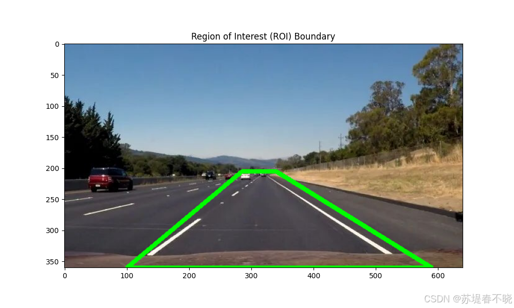
定义顶点：这里定义了一个梯形（四个坐标点，依次为左下，左上，右上，右下）。逻辑是：我们只关心图片下方大概车道所在的位置，天空、旁边的树木等区域的边缘对我们没用，需要过滤掉。
可视化部分 ：如果开关打开，就用 cv2.polylines 把这个梯形画在原图上并保存，方便确认框选的位置是否准确。

6. 应用掩膜（抠图）

python 复制代码

cv2.fillPoly(mask, vertices, ignore_mask_color)
masked_edges = cv2.bitwise_and(edges, mask)

填充多边形 ：把刚才定义的梯形区域在 mask 图上涂成白色（255），其他区域保持黑色。
按位与操作 ：将 edges（边缘图）和 mask（梯形白块）进行"与"运算。
效果：只保留了梯形区域内的边缘线条，梯形以外的边缘全部被清零（变黑）。

7. 霍夫变换 (Hough Transform) 参数设置

python 复制代码

rho = 1 
theta = np.pi/180 
threshold = 1     
min_line_length = 5 
max_line_gap = 1    
line_image = np.copy(image)*0

霍夫变换原理：将图像空间的直线映射到参数空间（极坐标系）来找线。
rho：距离分辨率，1表示网格步长为1像素。
theta：角度分辨率，这里是1度（π/180弧度）。
threshold ：投票门槛。设为 1 表示只要有 1 个点落在同一条参数线上，就认为这是一条直线（这个值设得非常小，通常为了检测短线条）。
min_line_length：过滤掉长度小于 5 像素的短线段。
max_line_gap：允许线段之间有最大 1 像素的断裂，依然把它们连成一条线。
line_image：创建一张纯黑的空白图，准备在上面画红线。

8. 执行霍夫变换并画线

python 复制代码

lines = cv2.HoughLinesP(masked_edges, rho, theta, threshold, np.array([]),
                            min_line_length, max_line_gap)

for line in lines:
    for x1,y1,x2,y2 in line:
        cv2.line(line_image,(x1,y1),(x2,y2),(255,0,0),10)

cv2.HoughLinesP ：概率霍夫变换，直接输出线段的起点 (x1,y1) 和终点 (x2,y2)。
循环画线 ：遍历检测到的所有线段，在黑色的 line_image 上用红色 (255,0,0)、粗细为 10 的线条把它们画出来。

9. 融合图像并保存结果

python 复制代码

color_edges = np.dstack((edges, edges, edges))

lines_edges = cv2.addWeighted(color_edges, 0.8, line_image, 1, 0)
plt.imshow(lines_edges)
plt.savefig('./demo/output1.png')

扩展通道 ：edges 原本是单通道灰度图，这里把它复制三份叠在一起变成三通道（看起来还是黑白的），以便能和彩色的线条图叠加。
加权融合 (addWeighted) ：公式为 dst = src1 * alpha + src2 * beta + gamma。
- 这里把边缘图权重设为 0.8，红线图权重设为 1。
- 效果：最终图片上既能看到淡淡的原图边缘轮廓，又能清晰地看到加粗红色的检测出的车道线。
保存：将最终结果保存为图片。

2、输出结果

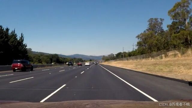
输入图片

设定的梯形区域

拟合出来的结果

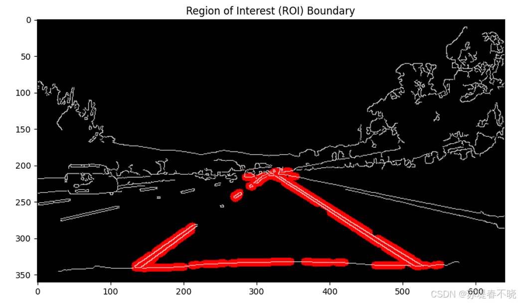
如果不设定梯形区域，也即

python 复制代码

vertices = np.array([[(0,imshape[0]),(0, 0), (imshape[1], 0), (imshape[1],imshape[0])]], dtype=np.int32)  # all image
# vertices = np.array([[(100,imshape[0]),(285, 205), (340, 205), (imshape[1]-50,imshape[0])]], dtype=np.int32)  # defining a quadrilateral region

得到的结果为

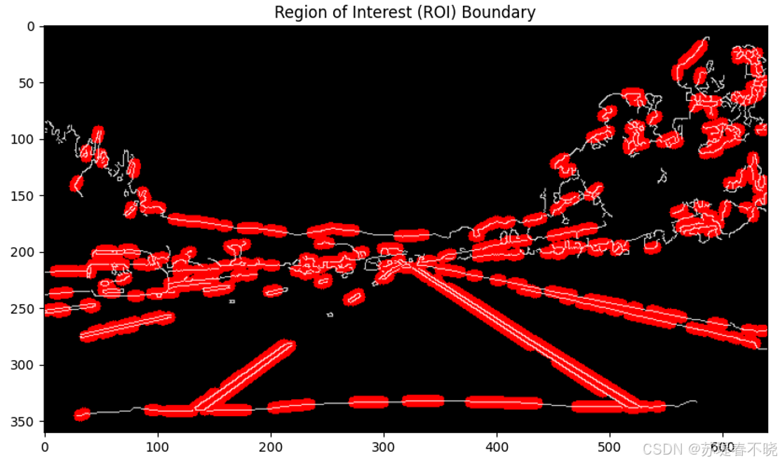
3、完整代码

py 复制代码

import matplotlib.pyplot as plt
import matplotlib.image as mpimg
import numpy as np
import cv2

plot_vertices = True
# Read in and grayscale the image
image = mpimg.imread('./demo/1.jpg')
gray = cv2.cvtColor(image,cv2.COLOR_RGB2GRAY)

# Define a kernel size and apply Gaussian smoothing
kernel_size = 5
blur_gray = cv2.GaussianBlur(gray,(kernel_size, kernel_size),0)

# Define our parameters for Canny and apply
low_threshold = 50
high_threshold = 150
edges = cv2.Canny(blur_gray, low_threshold, high_threshold)

# Next we'll create a masked edges image using cv2.fillPoly()
mask = np.zeros_like(edges)
ignore_mask_color = 255

# This time we are defining a four sided polygon to mask
imshape = image.shape
# vertices = np.array([[(0,imshape[0]),(0, 0), (imshape[1], 0), (imshape[1],imshape[0])]], dtype=np.int32)  # all image
vertices = np.array([[(100,imshape[0]),(285, 205), (340, 205), (imshape[1]-50,imshape[0])]], dtype=np.int32)  # defining a quadrilateral region

if plot_vertices:
    # 创建一个用于绘制 ROI 边界的图像副本
    roi_visualization = np.copy(image)

    # 将 vertices 转换为适合 cv2.polylines 的格式
    # isClosed=True 表示最后一点和第一点自动连接，形成封闭图形
    cv2.polylines(roi_visualization, [vertices], isClosed=True, color=(0, 255, 0), thickness=5)

    # 展示包含 ROI 框的图像
    plt.figure(figsize=(10, 6))
    plt.imshow(roi_visualization)
    plt.title('Region of Interest (ROI) Boundary')
    plt.savefig("./demo/vertices.png")

cv2.fillPoly(mask, vertices, ignore_mask_color)
masked_edges = cv2.bitwise_and(edges, mask)

# Define the Hough transform parameters
# Make a blank the same size as our image to draw on
rho = 1 # distance resolution in pixels of the Hough grid
theta = np.pi/180 # angular resolution in radians of the Hough grid
threshold = 1     # minimum number of votes (intersections in Hough grid cell)
min_line_length = 5 #minimum number of pixels making up a line
max_line_gap = 1    # maximum gap in pixels between connectable line segments
line_image = np.copy(image)*0 # creating a blank to draw lines on

# Run Hough on edge detected image
# Output "lines" is an array containing endpoints of detected line segments
lines = cv2.HoughLinesP(masked_edges, rho, theta, threshold, np.array([]),
                            min_line_length, max_line_gap)

# Iterate over the output "lines" and draw lines on a blank image
for line in lines:
    for x1,y1,x2,y2 in line:
        cv2.line(line_image,(x1,y1),(x2,y2),(255,0,0),10)

# Create a "color" binary image to combine with line image
color_edges = np.dstack((edges, edges, edges))

# Draw the lines on the edge image
lines_edges = cv2.addWeighted(color_edges, 0.8, line_image, 1, 0)
plt.imshow(lines_edges)
plt.savefig('./demo/output1.png')

# plt.show()

4、参考

python实现简单的车道线检测（2023-11-26）