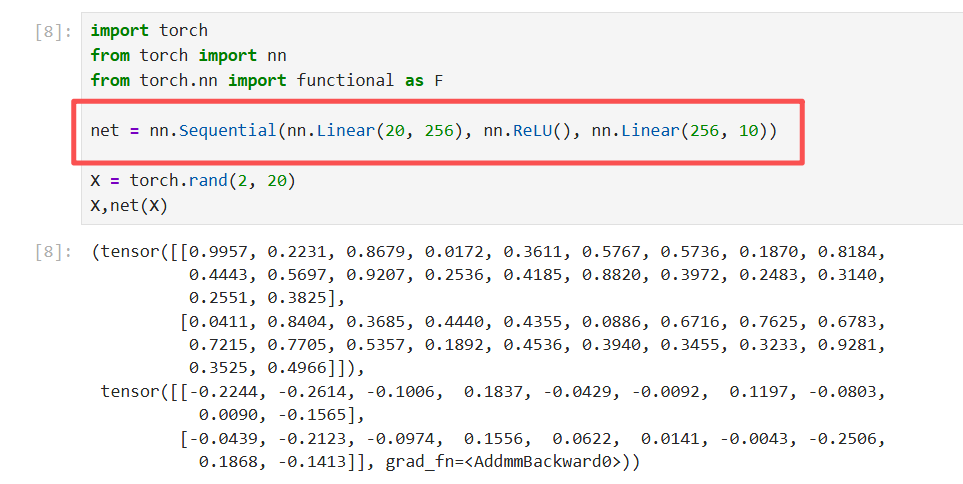
顺序块(下面也自定义了顺序快):
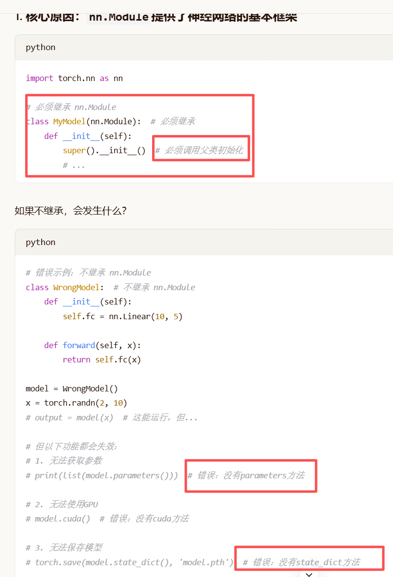
三种方式写 自定义块(需要继承nn.Module) 重点
不建议第二种 一般第一种简单
python
import torch.nn as nn
import torch.nn.functional as F

# 第一种方式:直接定义
class MLP1(nn.Module):
    def __init__(self):
        super().__init__()
        # 直接创建层
        self.hidden = nn.Linear(20, 256)
        self.relu = nn.ReLU()
        self.out = nn.Linear(256, 10)

    def forward(self, x):
        x = self.hidden(x)
        x = self.relu(x)
        x = self.out(x)
        return x

# 第二种方式:通过元组传入
class MLP2(nn.Module):
    def __init__(self, layers_tuple):
        super().__init__()
        # layers_tuple 是 (nn.Linear(20, 256), nn.ReLU(), nn.Linear(256, 10))
        # 我们需要在 __init__ 中处理这个元组
        self.layers = nn.ModuleList(layers_tuple)  # 使用ModuleList保存

    def forward(self, x):
        for layer in self.layers:
            x = layer(x)
        return x

# 第三种方式:自定义Sequential(更灵活)
class MySequential(nn.Module):
    def __init__(self, *args):  # 使用*args接收任意数量的参数
        super().__init__()
        # args 是一个元组,包含传入的所有层
# 这里,module是Module子类的一个实例。我们把它保存在'Module'类的成员
            # 变量_modules中。_module的类型是OrderedDict
        for idx, layer in enumerate(args):
            # 将每一层添加到 _modules 字典中
            self.add_module(str(idx), layer)
            # 或者:self._modules[str(idx)] = layer

    def forward(self, x):
        # 按顺序执行所有层 # OrderedDict保证了按照成员添加的顺序遍历它们
        for layer in self._modules.values():
            x = layer(x)
return x__init__函数将每个模块逐个添加到有序字典_modules 中。 读者可能会好奇为什么每个Module都有一个_modules属性? 以及为什么我们使用它而不是自己定义一个Python列表?
简而言之,_modules的主要优点是: 在模块的参数初始化过程中, 系统知道在_modules字典中查找需要初始化参数的子块。
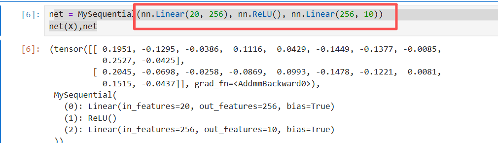
第三种方式调用:
X = torch.rand(2, 20)
创建一个形状为 (2, 20) 的张量,其中每个元素都是从均匀分布 U[0, 1) 中随机生成的浮点数。
why要自定义块:
Sequential类使模型构造变得简单, 允许我们组合新的架构,而不必定义自己的类。
然而,并不是所有的架构都是简单的顺序架构。 当需要更强的灵活性时,我们需要定义自己的块。 例如,我们可能希望在前向传播函数中执行Python的控制流。 此外,我们可能希望执行任意的数学运算, 而不是简单地依赖预定义的神经网络层。
参数共享:

from torch.nn import functional as F
python
# 对比两种写法:
# 写法A:参数共享(原始代码)
class SharedModel(nn.Module):
def __init__(self):
super().__init__()
self.linear = nn.Linear(20, 20) # 只有一组参数
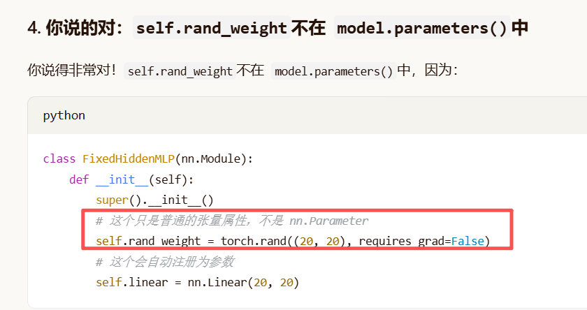
self.rand_weight = torch.rand((20, 20), requires_grad=False)
def forward(self, x):
x = self.linear(x) # 第一次使用
x = F.relu(torch.mm(x, self.rand_weight) + 1)
x = self.linear(x) # 第二次使用相同的参数
return x
# 写法B:不共享参数
class SeparateModel(nn.Module):
def __init__(self):
super().__init__()
self.linear1 = nn.Linear(20, 20) # 第一组参数
self.linear2 = nn.Linear(20, 20) # 第二组参数(不同的参数)
self.rand_weight = torch.rand((20, 20), requires_grad=False)
def forward(self, x):
x = self.linear1(x) # 使用linear1
x = F.relu(torch.mm(x, self.rand_weight) + 1)
x = self.linear2(x) # 使用linear2
return x
# 参数量对比
shared_model = SharedModel()
separate_model = SeparateModel()
print(f"参数共享模型参数量: {sum(p.numel() for p in shared_model.parameters())}")
print(f"独立参数模型参数量: {sum(p.numel() for p in separate_model.parameters())}")
# 输出:
# 参数共享模型参数量: 420 (20 * 20 + 20)
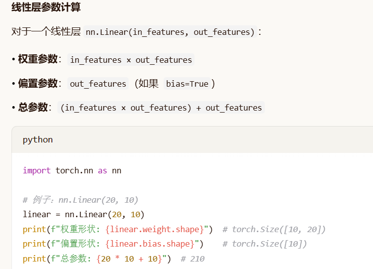
# 独立参数模型参数量: 840 (2*(20 * 20 + 20))参数量计算:
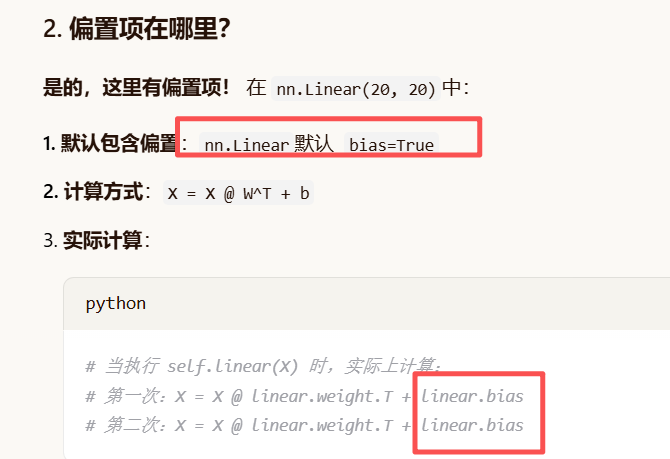
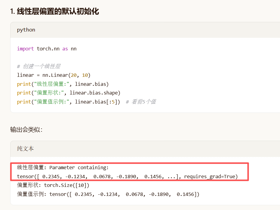
线性层默认的偏置(bias)不是0,而是随机初始化的。
验证:
上面例子的复用线性层的可训练参数计算:
步骤1:识别可训练参数
-
self.rand_weight:requires_grad=False,所以不算可训练参数 -
self.linear:这是可训练的参数-
权重:
20 × 20 = 400 -
偏置:
20 -
小计:
400 + 20 = 420
-
总可训练参数:420
步骤2:计算总参数(包括固定参数)
-
可训练参数:420
-
固定参数(
self.rand_weight):20 × 20 = 400 -
总参数 :
420 + 400 = 820
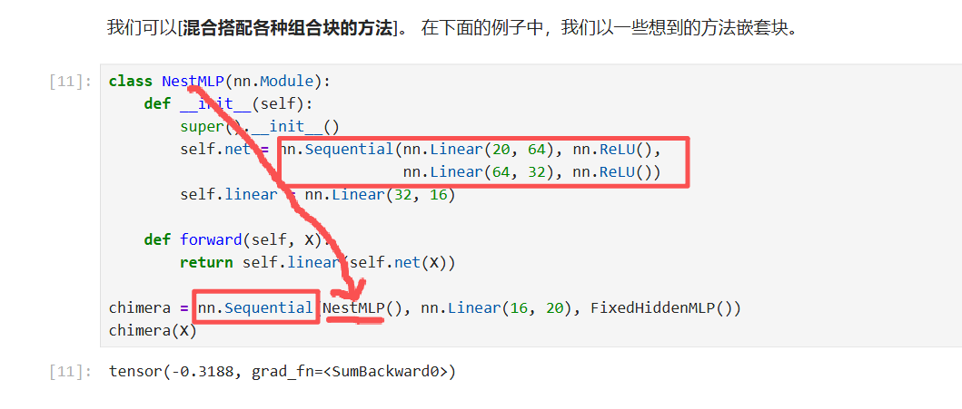
组合块: