R语言朴素贝叶斯算法---iris数据集

在R中，可通过e1071或caret包实现朴素贝叶斯，下面采用c1071实现。

R 复制代码

install.packages("e1071")  # 安装包
library(e1071)             # 加载包

数据集划分

R 复制代码

data(iris)
set.seed(123)
train_index <- sample(1:nrow(iris), 0.7 * nrow(iris))
train_data <- iris[train_index, ]        #训练集
test_data <- iris[-train_index, ]        #测试集

训练模型

R 复制代码

model <- naiveBayes(Species ~ ., data = train_data)

Naive Bayes Classifier for Discrete Predictors

Call:

naiveBayes.default(x = X, y = Y, laplace = laplace)

#先验概率，34%是山鸢尾，30%是变色鸢尾，35%是维吉尼亚鸢尾

A-priori probabilities:

setosa versicolor virginica

0.3428571 0.3047619 0.3523810

#条件概率，均值、标准差

#山鸢尾的花萼长度平均 4.97，波动小

#维吉尼亚鸢尾平均 6.59，明显更大

Conditional probabilities:

Sepal.Length

Y $,1$ $,2$

setosa 4.966667 0.3741657

versicolor 5.971875 0.4887340

virginica 6.586486 0.7165357

Sepal.Width

Y $,1$ $,2$

setosa 3.394444 0.4049299

versicolor 2.787500 0.3250310

virginica 2.948649 0.3500965

Petal.Length

Y $,1$ $,2$

setosa 1.461111 0.1777282

versicolor 4.309375 0.4423977

virginica 5.529730 0.6235494

Petal.Width

Y $,1$ $,2$

setosa 0.2555556 0.1157447

versicolor 1.3500000 0.1951013

virginica 1.9945946 0.2613490

预测与评估

R 复制代码

# 对测试集预测
pred <- predict(model, test_data)

# 查看前10个预测结果
head(pred, 10)

# 混淆矩阵
table(实际类别=test_data$Species, 预测类别=pred)

# 计算准确率
accuracy <- mean(pred == test_data$Species)
cat("模型准确率：", round(accuracy*100, 2), "%")

混淆矩阵

预测类别

实际类别 setosa versicolor virginica

setosa 14 0 0

versicolor 0 18 0

virginica 0 0 13

模型准确率： 100 %

参数调优

朴素贝叶斯的主要参数是拉普拉斯平滑（laplace），用于处理零概率问题。如果某个特征在某个类别里一次都没出现过 ，会算出： P(特征|类别) = 0，这个 0 会让整个分类概率直接变成 0 ，模型直接判断错误，出现零概率问题。

r 复制代码

model <- naiveBayes(Species ~ ., data = train_data, laplace = 1)

可视化

R 复制代码

library(ggplot2)

# 提取先验概率
prior <- data.frame(
  品种 = names(nb_model$apriori),
  概率 = as.numeric(nb_model$apriori)
)

# 画图
ggplot(prior, aes(x=品种, y=概率, fill=品种)) +
  geom_bar(stat="identity") +
  ggtitle("朴素贝叶斯：类别先验概率") +
  theme_minimal()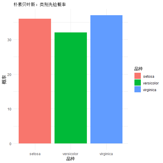

特征分布曲线

R 复制代码

#朴素贝叶斯假设连续特征服从高斯分布，模型存了均值和标准差，可以画出每条特征的分布曲线！
# 以 Sepal.Length 为例
ggplot(iris, aes(x=Sepal.Length, fill=Species)) +
  geom_density(alpha=0.5) +
  ggtitle("花萼长度在3个品种上的分布") +
  theme_minimal()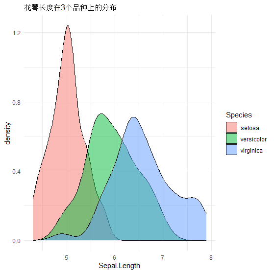

混淆矩阵热力图（模型准确率可视化）

R 复制代码

# 预测
pred <- predict(nb_model, test_data)
cm <- table(真实=test_data$Species, 预测=pred)

# 画热力图
heatmap(cm, col=heat.colors(10), scale="none", margins=c(10,10))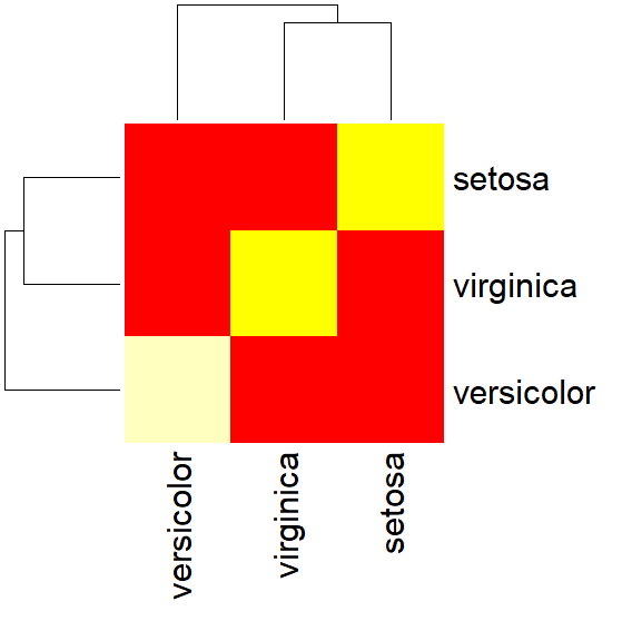

ggplot绘图

R 复制代码

library(ggplot2)
library(reshape2)

# 1. 生成预测与混淆矩阵
pred <- predict(nb_model, test_data)
cm <- table(真实 = test_data$Species, 预测 = pred)

# 2. 转成长格式（ggplot2必须）
cm_df <- melt(cm)

# 3. 画高颜值热力图（这是最标准的版本）
ggplot(cm_df, aes(x = 预测, y = 真实)) +
  geom_tile(aes(fill = value), color = "white", linewidth = 1) +  # 白色格子线
  scale_fill_gradient(low = "#F8F9FA", high = "#4285F4") +        # 蓝白渐变（谷歌风）
  geom_text(aes(label = value), size = 6, fontface = "bold") +    # 显示数字
  labs(
    title = "朴素贝叶斯 混淆矩阵",
    subtitle = "测试集预测结果",
    x = "预测类别",
    y = "真实类别",
    fill = "样本数量"
  ) +
  theme_minimal(base_size = 14) +
  theme(
    plot.title = element_text(hjust = 0.5),
    plot.subtitle = element_text(hjust = 0.5),
    axis.text = element_text(size = 12),
    axis.title = element_text(size = 13)
  ) +
  coord_fixed()  # 正方形格子，更好看

注意事项

特征独立性假设可能不成立，影响模型性能。
对连续型数据需离散化或假设分布（如高斯朴素贝叶斯）。
适用于高维数据，但需注意特征相关性。