AI基本结构12-lstm实现nlp

前序模型问题

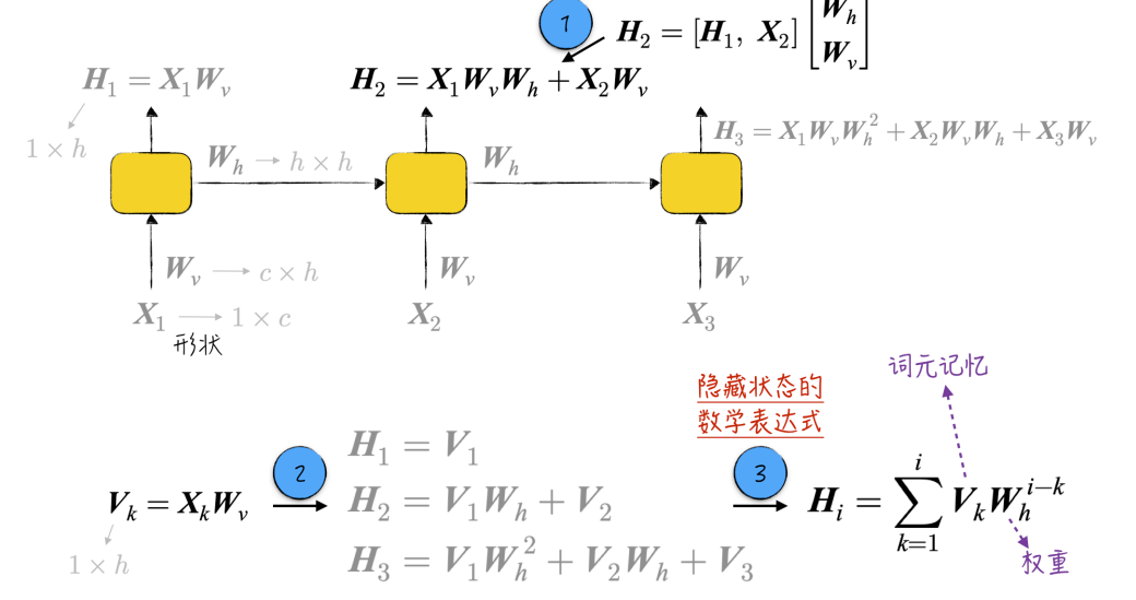
之前的深度循环神经网络CharRNNBatch虽然采用了两层 RNN，并引入了 LayerNorm 和 Dropout 提高训练稳定性，但其本质仍然是普通 RNN，因此仍然存在明显的短期记忆（Short-term Memory）问题，难以有效学习长距离依赖关系。

（1）隐藏状态的信息会逐渐衰减

RNN 利用隐藏状态（Hidden State）保存历史信息，每个时间步都会根据当前输入和上一时刻隐藏状态计算新的隐藏状态。然而，随着序列不断增长，早期信息需要经过多次状态更新才能传递到后面的时间步，在不断迭代过程中，早期信息会逐渐被新的信息覆盖，导致模型只能较好地保留最近几个时间步的信息，而较早的上下文容易遗失。

（2）梯度消失导致长期依赖难以学习

在反向传播过程中，误差需要沿时间维度逐步传播。当序列较长时，梯度经过连续的链式相乘容易不断减小，形成梯度消失，使模型难以更新与较早时间步相关的参数。因此，普通 RNN 更容易学习短期依赖，而难以捕捉跨越较长距离的语义关系。

LSTM

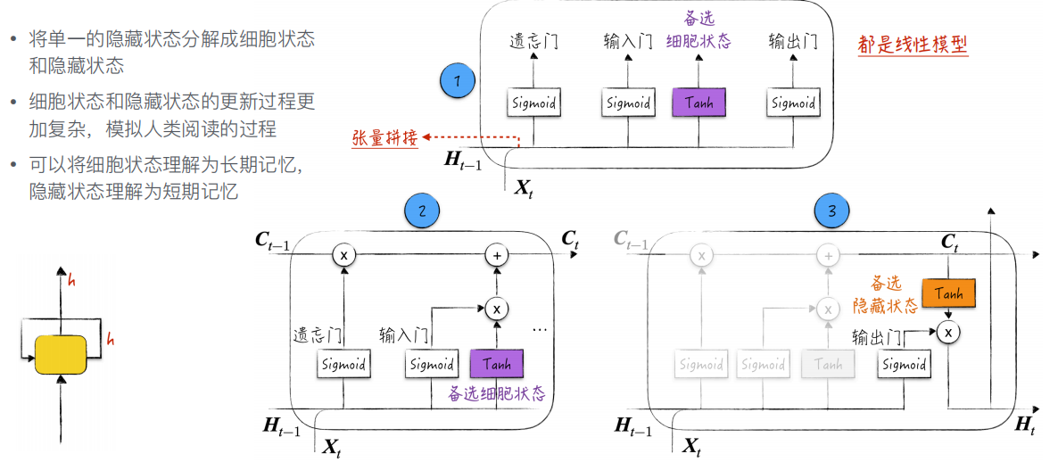
C保存长期记忆，H保存长期记忆，每轮从长期记忆基于遗忘门删去不需要的信息，再基于输入门取出可输入的长期记忆，再根据备选细胞状态选中需要更新的长期记忆，最后再根据新的长期记忆中被选中的部分输出短期内重要的信息输出。

ps:其余函数代码较上节基本没有修改

python 复制代码

class LSTMCell(nn.Module):

    def __init__(self, input_size, hidden_size):
        super().__init__()
        self.input_size = input_size
        self.hidden_size = hidden_size
        combined_size = hidden_size + input_size
        self.forget_gate = nn.Linear(combined_size, hidden_size)     # 遗忘门
        self.in_gate = nn.Linear(combined_size, hidden_size)         # 输入门
        self.new_cell_state = nn.Linear(combined_size, hidden_size)  # 备选细胞状态
        self.out_gate = nn.Linear(combined_size, hidden_size)        # 输出门

    def forward(self, input, state=None):
        # input: (B, I)
        # state: ((B, H), (B, H))
        B = input.shape[0]
        if state is None:
            state = self.init_state(B, input.device)
        hs, cs = state
        combined = torch.concat((input, hs), dim=-1)   # (B, I + H)
        # 细胞状态的更新
        ingate = F.sigmoid(self.in_gate(combined))
        forgetgate = F.sigmoid(self.forget_gate(combined))
        ncs = F.tanh(self.new_cell_state(combined))
        cs = (cs * forgetgate) + (ingate * ncs)
        # 隐藏状态的更新
        outgate = F.sigmoid(self.out_gate(combined))
        hs = F.tanh(cs) * outgate
        return hs, cs

    def init_state(self, B, device):
        hs = torch.zeros((B, self.hidden_size), device=device)
        cs = torch.zeros((B, self.hidden_size), device=device)
        return hs, cs
#测试
l_cell = LSTMCell(3, 4)
x = torch.randn(5, 3)
a, b = l_cell(x)
print(a.shape, b.shape)

（1）LSTMCell 的作用

LSTMCell 实现了一个最基本的 LSTM 单元，用于处理序列中的一个时间步数据。与普通 RnnCell 相比，它不仅维护隐藏状态（Hidden State，hs），还维护细胞状态（Cell State，cs），并通过门控机制控制信息的保留、更新和输出，从而增强长期记忆能力。

（2）网络结构

在初始化函数中，模型定义了四个全连接层，分别对应 LSTM 的四个核心部分：遗忘门（forget_gate）、输入门（in_gate）、备选细胞状态（new_cell_state）和输出门（out_gate）。由于每个门都需要同时利用当前输入和上一时刻隐藏状态，因此输入维度均为 input_size + hidden_size，输出维度为 hidden_size。

（3）状态初始化

forward() 函数首先判断是否提供了上一时刻状态 state。若为空，则调用 init_state() 初始化隐藏状态 hs 和细胞状态 cs，两者均为全零张量，作为序列开始时的初始记忆。

（4）细胞状态更新

模型首先将当前输入与上一时刻隐藏状态拼接，然后分别计算输入门、遗忘门和备选细胞状态。其中，输入门和遗忘门通过 Sigmoid 输出 0～1 的权重，控制信息保留比例；备选细胞状态通过 tanh 生成新的候选记忆。最终利用公式

更新细胞状态，实现"遗忘旧信息、加入新信息"的过程。

（5）隐藏状态更新

细胞状态更新完成后，再计算输出门。输出门同样经过 Sigmoid 得到权重，然后将细胞状态经过 tanh 激活，并与输出门相乘，得到新的隐藏状态：

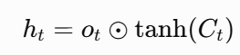
隐藏状态既作为当前时间步的输出，也会传递到下一时间步继续参与计算。

python 复制代码

class LSTM(nn.Module):

    def __init__(self, input_size, hidden_size):
        super().__init__()
        self.cell = LSTMCell(input_size, hidden_size)

    def forward(self, input, state=None):
        # input:  (B, T, C)
        # state:  ((B, H), (B, H))
        # out:    (B, T, H)
        B, T, C = input.shape
        re = []
        for i in range(T):
            state = self.cell(input[:, i, :], state)
            re.append(state[0])
        return torch.stack(re, dim=1)     # (B, T, H)

LSTM 类是在 LSTMCell 的基础上封装得到的完整序列模型，用于处理整个输入序列，而不仅仅是单个时间步。输入数据形状为 (B, T, C)，其中 B 表示批量大小、T 表示序列长度、C 表示输入特征维度。模型内部利用 for 循环依次取出每个时间步的数据，并调用 LSTMCell 更新隐藏状态和细胞状态；每一步产生的隐藏状态都会保存到列表中，最后通过 torch.stack(re, dim=1) 拼接成形状为 (B, T, H) 的输出，表示整个序列所有时间步的隐藏状态。与 LSTMCell 只能处理一个时间步不同，LSTM 能够自动完成整个序列的循环计算，更适合直接用于序列建模和训练。

python 复制代码

class CharLSTM(nn.Module):
    def __init__(self, vs):
        super().__init__()
        self.emb_size = 256
        self.hidden_size = 128
        self.emb = nn.Embedding(vs, self.emb_size)
        self.dp = nn.Dropout(0.4)
        self.lstm1 = LSTM(self.emb_size, self.hidden_size)
        self.ln1 = nn.LayerNorm(self.hidden_size)
        self.lstm2 = LSTM(self.hidden_size, self.hidden_size)
        self.ln2 = nn.LayerNorm(self.hidden_size)
        self.lstm3 = LSTM(self.hidden_size, self.hidden_size)
        self.ln3 = nn.LayerNorm(self.hidden_size)
        self.lm = nn.Linear(self.hidden_size, vs)
    def forward(self, x):
        # x: (B, T)
        embeddings = self.emb(x)   # (B, T, C)
        h = self.ln1(self.dp(self.lstm1(embeddings)))  # (B, T, H)
        h = self.ln2(self.dp(self.lstm2(h)))           # (B, T, H)
        h = self.ln3(self.dp(self.lstm3(h)))           # (B, T, H)
        output = self.lm(h)
        return output
#测试
c_model = CharLSTM(len(tokenizer.char2ind)).to(device)
context = torch.tensor(tokenizer.encode('def'), device=device).unsqueeze(0)
print(''.join(tokenizer.decode(generate(c_model, context, tokenizer))))
print(estimate_loss(c_model))
l = train_model(c_model, optim.Adam(c_model.parameters(), lr=learning_rate))
context = torch.tensor(tokenizer.encode('def'), device=device).unsqueeze(0)
print(''.join(tokenizer.decode(generate(c_model, context, tokenizer))))

1）模型整体结构

CharLSTM 是一个字符级长短期记忆网络（LSTM）语言模型，整体采用 Embedding → LSTM → Dropout → LayerNorm → LSTM → Dropout → LayerNorm → LSTM → Dropout → LayerNorm → Linear 的结构。模型首先将字符编号映射为向量，再利用三层 LSTM 提取序列特征，最后通过全连接层输出每个时间步对词表中所有字符的预测结果。

（2）Embedding

Embedding 层将离散的字符编号转换为 256 维稠密向量，使模型能够学习字符之间的语义关系，为后续 LSTM 提供连续的特征表示。

（3）三层 LSTM 特征提取

模型连续堆叠了三层 LSTM，每层都能够利用门控机制保存长期信息、过滤无关信息，并学习更加复杂的上下文特征。随着层数增加，模型能够逐步提取从低层字符特征到高层语义特征，提高文本建模能力。

（4）Dropout 与 LayerNorm

每层 LSTM 后都加入 Dropout(0.4) 和 LayerNorm。其中，Dropout 随机屏蔽部分神经元，减少过拟合；LayerNorm 对每个时间步的隐藏特征进行归一化，使数据分布更加稳定，加快模型收敛，并进一步提高训练稳定性。