文章目录
贝尔曼期望方程
给定一个固定策略 π,贝尔曼期望方程为
V π ( s ) = Σ a π ( a ∣ s ) ∗ R ( s , a ) + γ ∗ Σ s ′ P ( s ′ ∣ s , a ) ∗ V π ( s ′ ) V^π(s) = Σ_a π(a|s) * R(s,a) + γ \* Σ_{s'} P(s'\|s,a) \* V\^π(s') Vπ(s)=Σaπ(a∣s)∗R(s,a)+γ∗Σs′P(s′∣s,a)∗Vπ(s′)
- 贝尔曼最优方程
V ∗ ( s ) = max a Σ s ′ P ( s ′ ∣ s , a ) R ( s , a ) + γ V ∗ ( s ′ ) V^*(s) = \max_a Σ_{s'} P(s'|s,a) R(s,a) + γ V\^\*(s') V∗(s)=amaxΣs′P(s′∣s,a)R(s,a)+γV∗(s′)
python
"""
第3章:贝尔曼方程的数值验证
用代码验证贝尔曼期望方程和贝尔曼最优方程

本实验展示:
1. 手工计算贝尔曼期望方程 V^π(s)
2. 用价值迭代(Value Iteration)数值求解 V^π(s) 和 V*(s)
3. 对比两种方法的结果,验证一致性
4. 展示价值迭代逐步收敛的过程

运行方式:
    python bellman_equation_verify.py
"""

import os
import numpy as np
import matplotlib.pyplot as plt

# 创建输出目录
os.makedirs("output", exist_ok=True)


# ==========================================
# 第一部分:定义一个简单的 3 状态 MDP
# ==========================================
# 我们手工构造一个微型 MDP,方便手工计算和代码验证。
#
# 状态集合:S = {s0, s1, s2}
# 动作集合:A = {a0, a1}(每个状态可选两个动作)
#
# 转移概率 P(s'|s,a) 和奖励 R(s,a) 定义如下:
#
# 从 s0 出发:
#   执行 a0 → 转移到 s1(概率 1.0),奖励 = 1
#   执行 a1 → 转移到 s2(概率 1.0),奖励 = 2
#
# 从 s1 出发:
#   执行 a0 → 转移到 s0(概率 0.5),奖励 = -1
#                 转移到 s2(概率 0.5),奖励 = -1
#   执行 a1 → 转移到 s1(概率 0.8),奖励 = 0
#                 转移到 s2(概率 0.2),奖励 = 0
#
# 从 s2 出发:
#   执行 a0 → 转移到 s1(概率 1.0),奖励 = 3
#   执行 a1 → 转移到 s2(概率 1.0),奖励 = 1(自循环)

# 状态和动作数量
N_STATES = 3
N_ACTIONS = 2

# 转移概率:P[s][a] = {下一状态: 概率}
P = {
    0: {  # s0
        0: {1: 1.0},    # a0 → s1 概率 1.0
        1: {2: 1.0},    # a1 → s2 概率 1.0
    },
    1: {  # s1
        0: {0: 0.5, 2: 0.5},  # a0 → s0 概率 0.5, s2 概率 0.5
        1: {1: 0.8, 2: 0.2},  # a1 → s1 概率 0.8, s2 概率 0.2
    },
    2: {  # s2
        0: {1: 1.0},    # a0 → s1 概率 1.0
        1: {2: 1.0},    # a1 → s2 概率 1.0(自循环)
    },
}

# 奖励函数:R[s][a] = 立即奖励
R = {
    0: {0: 1, 1: 2},     # s0: a0 奖励 1, a1 奖励 2
    1: {0: -1, 1: 0},    # s1: a0 奖励 -1, a1 奖励 0
    2: {0: 3, 1: 1},     # s2: a0 奖励 3, a1 奖励 1
}

GAMMA = 0.9  # 折扣因子


# ==========================================
# 第二部分:贝尔曼期望方程 ------ 手工计算
# ==========================================
def manual_bellman_expectation():
    """
    手工计算贝尔曼期望方程 V^π(s)

    给定一个固定策略 π,贝尔曼期望方程为:
        V^π(s) = Σ_a π(a|s) * [R(s,a) + γ * Σ_{s'} P(s'|s,a) * V^π(s')]

    我们使用一个简单的均匀随机策略:
        π(a|s) = 0.5(每个动作等概率选择)

    手工推导(令 V^π(s0) = v0, V^π(s1) = v1, V^π(s2) = v2):

    V^π(s0) = 0.5 * [R(s0,a0) + γ * V^π(s1)] + 0.5 * [R(s0,a1) + γ * V^π(s2)]
            = 0.5 * [1 + 0.9 * v1] + 0.5 * [2 + 0.9 * v2]
            = 0.5 + 0.45*v1 + 1 + 0.45*v2
            = 1.5 + 0.45*v1 + 0.45*v2  ........................ (方程1)

    V^π(s1) = 0.5 * [R(s1,a0) + γ * (0.5*V^π(s0) + 0.5*V^π(s2))]
            + 0.5 * [R(s1,a1) + γ * (0.8*V^π(s1) + 0.2*V^π(s2))]
            = 0.5 * [-1 + 0.9*(0.5*v0 + 0.5*v2)]
            + 0.5 * [0 + 0.9*(0.8*v1 + 0.2*v2)]
            = -0.5 + 0.225*v0 + 0.225*v2 + 0.36*v1 + 0.09*v2
            = -0.5 + 0.225*v0 + 0.36*v1 + 0.315*v2  ............ (方程2)

    V^π(s2) = 0.5 * [R(s2,a0) + γ * V^π(s1)] + 0.5 * [R(s2,a1) + γ * V^π(s2)]
            = 0.5 * [3 + 0.9 * v1] + 0.5 * [1 + 0.9 * v2]
            = 1.5 + 0.45*v1 + 0.5 + 0.45*v2
            = 2.0 + 0.45*v1 + 0.45*v2  ........................ (方程3)
    """
    print("=" * 60)
    print("  贝尔曼期望方程 ------ 手工推导")
    print("=" * 60)
    print()
    print("给定策略:均匀随机 π(a|s) = 0.5")
    print(f"折扣因子:γ = {GAMMA}")
    print()
    print("列方程组(v0 = V^π(s0), v1 = V^π(s1), v2 = V^π(s2)):")
    print("  v0 = 1.5   + 0.45*v1 + 0.45*v2  ...... (方程1)")
    print("  v1 = -0.5  + 0.225*v0 + 0.36*v1 + 0.315*v2  (方程2)")
    print("  v2 = 2.0   + 0.45*v1 + 0.45*v2  ...... (方程3)")
    print()

    # 求解线性方程组 A * v = b
    # 方程1: v0 - 0.45*v1 - 0.45*v2 = 1.5
    # 方程2: -0.225*v0 + (1-0.36)*v1 - 0.315*v2 = -0.5
    # 方程3: -0.45*v1 + (1-0.45)*v2 = 2.0

    A = np.array([
        [1.0,   -0.45,   -0.45],
        [-0.225, 0.64,   -0.315],
        [0.0,   -0.45,    0.55],
    ])
    b = np.array([1.5, -0.5, 2.0])

    manual_V = np.linalg.solve(A, b)

    print("手工求解线性方程组得到:")
    for i in range(N_STATES):
        print(f"  V^π(s{i}) = {manual_V[i]:.6f}")
    print()
    return manual_V


# ==========================================
# 第三部分:策略评估 ------ 迭代求解贝尔曼期望方程
# ==========================================
def policy_evaluation(policy, max_iter=1000, tol=1e-8):
    """
    策略评估:通过迭代求解贝尔曼期望方程

    贝尔曼期望方程(迭代形式):
        V(s) ← Σ_a π(a|s) * [R(s,a) + γ * Σ_{s'} P(s'|s,a) * V(s')]

    反复迭代直到 V(s) 收敛,收敛后的 V(s) 就是 V^π(s)。

    参数:
        policy: 策略 π(a|s),形状 (N_STATES, N_ACTIONS)
        max_iter: 最大迭代次数
        tol: 收敛阈值
    返回:
        V: 状态价值函数
        history: 每次迭代的 V 值记录(用于可视化收敛过程)
    """
    V = np.zeros(N_STATES)
    history = [V.copy()]

    for iteration in range(max_iter):
        V_new = np.zeros(N_STATES)

        for s in range(N_STATES):
            # 贝尔曼期望方程:对所有动作求加权和
            for a in range(N_ACTIONS):
                # π(a|s) * [R(s,a) + γ * Σ P(s'|s,a) * V(s')]
                action_value = R[s][a]
                for next_s, prob in P[s][a].items():
                    action_value += GAMMA * prob * V[next_s]
                V_new[s] += policy[s][a] * action_value

        # 检查是否收敛
        delta = np.max(np.abs(V_new - V))
        history.append(V_new.copy())
        V = V_new

        if delta < tol:
            break

    return V, history


# ==========================================
# 第四部分:价值迭代 ------ 求解贝尔曼最优方程
# ==========================================
def value_iteration(max_iter=1000, tol=1e-8):
    """
    价值迭代:求解贝尔曼最优方程,找到 V*(s)

    贝尔曼最优方程(迭代形式):
        V(s) ← max_a [R(s,a) + γ * Σ_{s'} P(s'|s,a) * V(s')]

    与贝尔曼期望方程的区别:
    - 期望方程:给定策略 π,求 V^π(s)
    - 最优方程:对所有策略取最优,求 V*(s)

    V*(s) 满足:
        V*(s) = max_a Σ_{s'} P(s'|s,a) [R(s,a) + γ * V*(s')]

    参数:
        max_iter: 最大迭代次数
        tol: 收敛阈值
    返回:
        V_star: 最优状态价值函数
        optimal_policy: 最优策略
        history: 收敛过程
    """
    V = np.zeros(N_STATES)
    history = [V.copy()]

    for iteration in range(max_iter):
        V_new = np.zeros(N_STATES)

        for s in range(N_STATES):
            # 对每个动作计算 Q(s, a)
            q_values = []
            for a in range(N_ACTIONS):
                q = R[s][a]
                for next_s, prob in P[s][a].items():
                    q += GAMMA * prob * V[next_s]
                q_values.append(q)

            # 贝尔曼最优方程:取最大值而不是期望
            V_new[s] = max(q_values)

        delta = np.max(np.abs(V_new - V))
        history.append(V_new.copy())
        V = V_new

        if delta < tol:
            break

    # 从 V* 提取最优策略
    optimal_policy = extract_optimal_policy(V)

    return V, optimal_policy, history


def extract_optimal_policy(V):
    """
    从最优价值函数 V* 提取最优策略 π*

    π*(s) = argmax_a [R(s,a) + γ * Σ_{s'} P(s'|s,a) * V*(s')]
    """
    policy = np.zeros((N_STATES, N_ACTIONS))

    for s in range(N_STATES):
        q_values = []
        for a in range(N_ACTIONS):
            q = R[s][a]
            for next_s, prob in P[s][a].items():
                q += GAMMA * prob * V[next_s]
            q_values.append(q)

        best_action = np.argmax(q_values)
        policy[s][best_action] = 1.0  # 确定性策略

    return policy


# ==========================================
# 第五部分:结果对比与可视化
# ==========================================
def verify_results():
    """验证手工计算与迭代计算的一致性"""

    # 均匀随机策略
    uniform_policy = np.ones((N_STATES, N_ACTIONS)) / N_ACTIONS

    print("=" * 60)
    print("  贝尔曼方程数值验证")
    print("=" * 60)
    print()

    # ------------------------------------------
    # 对比1:手工计算 vs 迭代求解(贝尔曼期望方程)
    # ------------------------------------------
    print("-" * 60)
    print("  对比1:贝尔曼期望方程 V^π(s) 的两种求解方式")
    print("-" * 60)

    # 手工计算
    manual_V = manual_bellman_expectation()

    # 迭代计算
    iter_V, iter_history = policy_evaluation(uniform_policy)
    print("策略评估(迭代求解)结果:")
    for i in range(N_STATES):
        print(f"  V^π(s{i}) = {iter_V[i]:.6f}")
    print()

    # 对比
    print(">>> 对比结果:")
    print(f"  {'状态':<8s} {'手工计算':<15s} {'迭代求解':<15s} {'误差':<15s}")
    for i in range(N_STATES):
        error = abs(manual_V[i] - iter_V[i])
        print(f"  s{i:<6d} {manual_V[i]:<15.8f} {iter_V[i]:<15.8f} {error:<15.2e}")

    all_match = np.allclose(manual_V, iter_V, atol=1e-6)
    print(f"\n  结论:{'完全一致 ✓' if all_match else '存在差异 ✗'}")
    print(f"  (手工求解线性方程组 = 迭代法逐步收敛,殊途同归!)")
    print()

    # ------------------------------------------
    # 对比2:贝尔曼期望方程 vs 贝尔曼最优方程
    # ------------------------------------------
    print("-" * 60)
    print("  对比2:V^π(s) vs V*(s)")
    print("-" * 60)
    print()

    V_star, optimal_policy, vi_history = value_iteration()

    print("贝尔曼期望方程 V^π(s)(均匀随机策略下):")
    for i in range(N_STATES):
        print(f"  V^π(s{i}) = {iter_V[i]:.6f}")

    print()
    print("贝尔曼最优方程 V*(s)(最优策略下):")
    for i in range(N_STATES):
        print(f"  V*(s{i}) = {V_star[i]:.6f}")

    print()
    print("最优策略 π*:")
    action_names = ['a0', 'a1']
    for s in range(N_STATES):
        best = np.argmax(optimal_policy[s])
        print(f"  π*(s{s}) = {action_names[best]}")

    print()
    print(f"  {'状态':<8s} {'V^π(s) 随机策略':<20s} {'V*(s) 最优策略':<20s} {'提升':<10s}")
    for i in range(N_STATES):
        improvement = V_star[i] - iter_V[i]
        print(f"  s{i:<6d} {iter_V[i]:<20.6f} {V_star[i]:<20.6f} {improvement:>+10.6f}")

    print()
    print("  分析:V*(s) ≥ V^π(s) 对所有状态成立(最优策略不会更差)")

    # ------------------------------------------
    # 可视化:价值迭代收敛过程
    # ------------------------------------------
    visualize_convergence(iter_history, vi_history)


def visualize_convergence(expectation_history, optimal_history):
    """
    可视化价值迭代的收敛过程

    左图:策略评估(贝尔曼期望方程)的收敛过程
    右图:价值迭代(贝尔曼最优方程)的收敛过程
    """
    plt.rcParams['font.sans-serif'] = ['Arial Unicode MS', 'SimHei']
    plt.rcParams['axes.unicode_minus'] = False

    fig, axes = plt.subplots(1, 2, figsize=(14, 5))

    # ------------------------------------------
    # 左图:贝尔曼期望方程收敛过程
    # ------------------------------------------
    ax1 = axes[0]
    history_arr = np.array(expectation_history)
    colors = ['#e74c3c', '#2ecc71', '#3498db']
    state_labels = ['V^π(s0)', 'V^π(s1)', 'V^π(s2)']

    for s in range(N_STATES):
        ax1.plot(history_arr[:, s], color=colors[s], label=state_labels[s], linewidth=2)

    ax1.set_xlabel('迭代次数', fontsize=11)
    ax1.set_ylabel('状态价值 V(s)', fontsize=11)
    ax1.set_title('策略评估收敛过程\n(贝尔曼期望方程)', fontsize=12)
    ax1.legend(fontsize=10)
    ax1.grid(True, alpha=0.3)

    # 只显示前 30 次迭代(后面的已经收敛)
    n_show = min(30, len(expectation_history))
    ax1.set_xlim(0, n_show)

    # ------------------------------------------
    # 右图:贝尔曼最优方程收敛过程
    # ------------------------------------------
    ax2 = axes[1]
    history_arr2 = np.array(optimal_history)

    state_labels_star = ['V*(s0)', 'V*(s1)', 'V*(s2)']
    for s in range(N_STATES):
        ax2.plot(history_arr2[:, s], color=colors[s], label=state_labels_star[s], linewidth=2)

    ax2.set_xlabel('迭代次数', fontsize=11)
    ax2.set_ylabel('状态价值 V(s)', fontsize=11)
    ax2.set_title('价值迭代收敛过程\n(贝尔曼最优方程)', fontsize=12)
    ax2.legend(fontsize=10)
    ax2.grid(True, alpha=0.3)

    n_show2 = min(30, len(optimal_history))
    ax2.set_xlim(0, n_show2)

    plt.tight_layout()
    plt.savefig('output/bellman_equation_verify_results.png', dpi=150, bbox_inches='tight')
    print("\n图表已保存至 output/bellman_equation_verify_results.png")
    plt.show()


# ==========================================
# 第六部分:逐步展示价值迭代过程
# ==========================================
def print_value_iteration_steps(n_steps=10):
    """
    打印价值迭代的前 n_steps 步,展示逐步收敛的过程

    这让读者能直观看到:
    - 初始时 V(s) = 0(什么都不知道)
    - 每一步,V(s) 通过贝尔曼方程更新,向真实值逼近
    - 经过足够多步后,V(s) 收敛到最优值
    """
    print()
    print("=" * 60)
    print("  价值迭代逐步收敛过程")
    print("=" * 60)
    print()
    print("  迭代  |  V*(s0)    V*(s1)    V*(s2)   |  最大变化")
    print("  " + "-" * 55)

    V = np.zeros(N_STATES)

    for iteration in range(n_steps):
        V_new = np.zeros(N_STATES)

        for s in range(N_STATES):
            q_values = []
            for a in range(N_ACTIONS):
                q = R[s][a]
                for next_s, prob in P[s][a].items():
                    q += GAMMA * prob * V[next_s]
                q_values.append(q)
            V_new[s] = max(q_values)

        delta = np.max(np.abs(V_new - V))

        print(f"  {iteration + 1:4d}  |"
              f"  {V_new[0]:>8.4f}  {V_new[1]:>8.4f}  {V_new[2]:>8.4f} |"
              f"  {delta:>8.6f}")

        V = V_new

        if delta < 1e-8:
            print(f"\n  在第 {iteration + 1} 步收敛!")
            break

    print("  " + "-" * 55)
    print(f"\n  最终最优状态价值函数:")
    for i in range(N_STATES):
        print(f"    V*(s{i}) = {V[i]:.6f}")

    # 打印最优策略
    print(f"\n  最优策略:")
    action_names = ['a0', 'a1']
    for s in range(N_STATES):
        q_values = []
        for a in range(N_ACTIONS):
            q = R[s][a]
            for next_s, prob in P[s][a].items():
                q += GAMMA * prob * V[next_s]
            q_values.append(q)
        best = np.argmax(q_values)
        print(f"    π*(s{s}) = {action_names[best]}  "
              f"(Q(s{s},a0)={q_values[0]:.4f}, Q(s{s},a1)={q_values[1]:.4f})")


# ==========================================
# 主程序
# ==========================================
def main():
    """主函数:运行所有验证实验"""

    # 1. 验证手工计算与迭代计算的一致性
    verify_results()

    # 2. 展示价值迭代逐步收敛
    print_value_iteration_steps(n_steps=20)


if __name__ == "__main__":
    main()
python
============================================================
  贝尔曼方程数值验证
============================================================

------------------------------------------------------------
  对比1:贝尔曼期望方程 V^π(s) 的两种求解方式
------------------------------------------------------------
============================================================
  贝尔曼期望方程 ------ 手工推导
============================================================

给定策略:均匀随机 π(a|s) = 0.5
折扣因子:γ = 0.9

列方程组(v0 = V^π(s0), v1 = V^π(s1), v2 = V^π(s2)):
  v0 = 1.5   + 0.45*v1 + 0.45*v2  ...... (方程1)
  v1 = -0.5  + 0.225*v0 + 0.36*v1 + 0.315*v2  (方程2)
  v2 = 2.0   + 0.45*v1 + 0.45*v2  ...... (方程3)

手工求解线性方程组得到:
  V^π(s0) = 8.714450
  V^π(s1) = 6.817661
  V^π(s2) = 9.214450

策略评估(迭代求解)结果:
  V^π(s0) = 8.714449
  V^π(s1) = 6.817660
  V^π(s2) = 9.214449

>>> 对比结果:
  状态       手工计算            迭代求解            误差
  s0      8.71444954      8.71444945      8.81e-08
  s1      6.81766055      6.81766046      8.81e-08
  s2      9.21444954      9.21444945      8.81e-08

  结论:完全一致 ✓
  (手工求解线性方程组 = 迭代法逐步收敛,殊途同归!)

------------------------------------------------------------
  对比2:V^π(s) vs V*(s)
------------------------------------------------------------

贝尔曼期望方程 V^π(s)(均匀随机策略下):
  V^π(s0) = 8.714449
  V^π(s1) = 6.817660
  V^π(s2) = 9.214449

贝尔曼最优方程 V*(s)(最优策略下):
  V*(s0) = 13.362256
  V*(s1) = 10.694143
  V*(s2) = 12.624729

最优策略 π*:
  π*(s0) = a1
  π*(s1) = a0
  π*(s2) = a0

  状态       V^π(s) 随机策略          V*(s) 最优策略           提升
  s0      8.714449             13.362256             +4.647806
  s1      6.817660             10.694143             +3.876483
  s2      9.214449             12.624729             +3.410279

  分析:V*(s) ≥ V^π(s) 对所有状态成立(最优策略不会更差)

图表已保存至 output/bellman_equation_verify_results.png

============================================================
  价值迭代逐步收敛过程
============================================================

  迭代  |  V*(s0)    V*(s1)    V*(s2)   |  最大变化
  -------------------------------------------------------
     1  |    2.0000    0.0000    3.0000 |  3.000000
     2  |    4.7000    1.2500    3.7000 |  2.700000
     3  |    5.3300    2.7800    4.3300 |  1.530000
     4  |    5.8970    3.3470    5.5020 |  1.172000
     5  |    6.9518    4.1296    6.0123 |  1.054800
     6  |    7.4111    4.8338    6.7166 |  0.704295
     7  |    8.0449    5.3574    7.3505 |  0.633866
     8  |    8.6154    5.9279    7.8217 |  0.570479
     9  |    9.0395    6.3967    8.3351 |  0.513431
    10  |    9.5016    6.8186    8.7570 |  0.462088
    11  |    9.8813    7.2164    9.1367 |  0.397794
    12  |   10.2231    7.5581    9.4948 |  0.358014
    13  |   10.5453    7.8730    9.8023 |  0.322213
    14  |   10.8221    8.1564   10.0857 |  0.283399
    15  |   11.0771    8.4085   10.3408 |  0.255059
    16  |   11.3067    8.6381   10.5677 |  0.229553
    17  |   11.5109    8.8435   10.7743 |  0.206598
    18  |   11.6968    9.0283   10.9591 |  0.185938
    19  |   11.8632    9.1952   11.1255 |  0.166858
    20  |   12.0129    9.3449   11.2757 |  0.150172
  -------------------------------------------------------

  最终最优状态价值函数:
    V*(s0) = 12.012939
    V*(s1) = 9.344911
    V*(s2) = 11.275659

  最优策略:
    π*(s0) = a1  (Q(s0,a0)=9.4104, Q(s0,a1)=12.1481)
    π*(s1) = a0  (Q(s1,a0)=9.4799, Q(s1,a1)=8.7580)
    π*(s2) = a0  (Q(s2,a0)=11.4104, Q(s2,a1)=11.1481)
Q-learning
Q-Learning 的核心更新公式(贝尔曼最优方程的迭代形式):
Q ( s , a ) ← Q ( s , a ) + α ∗ r + γ ∗ max a ′ Q ( s ′ , a ′ ) − Q ( s , a ) Q(s, a) ← Q(s, a) + α * r + γ \*\\max_{a'} Q(s', a') - Q(s, a) Q(s,a)←Q(s,a)+α∗r+γ∗a′maxQ(s′,a′)−Q(s,a)
其中:
    - s: 当前状态
    - a: 当前动作
    - r: 获得的奖励
    - s': 下一个状态
    - α: 学习率(控制更新步长)
    - γ: 折扣因子(未来奖励的重要程度)
    - max_a' Q(s', a'): 下一个状态的最大 Q 值
python
"""
第3章:4×4 GridWorld Q-Learning 实验
在网格世界中学习最优路径,直观理解 Q 值和贝尔曼方程

运行方式:
    python gridworld_q_learning.py
"""

import os
import numpy as np
import matplotlib.pyplot as plt

# 创建输出目录
os.makedirs("output", exist_ok=True)


# ==========================================
# 第一部分:GridWorld 环境
# ==========================================
class GridWorld:
    """
    4×4 网格世界环境

    网格布局(4行4列):
        0,0  0,1  0,2  0,3
        1,0  1,1  1,2  1,3
        2,0  2,1  2,2  2,3
        3,0  3,1  3,2  3,3

    - 起点:(0, 0)
    - 终点:(3, 3),到达获得 +10 奖励
    - 障碍物:(1, 1) 和 (2, 2),撞到获得 -5 惩罚
    - 每走一步:-1 奖励(鼓励尽快到达终点)
    - 撞墙:-5 奖励(位置不变)

    动作空间:
        0 = 上 (↑), 1 = 下 (↓), 2 = 左 (←), 3 = 右 (→)
    """

    def __init__(self):
        self.rows = 4
        self.cols = 4
        self.start = (0, 0)
        self.goal = (3, 3)
        self.obstacles = [(1, 1), (2, 2)]
        self.n_actions = 4  # 上、下、左、右
        self.action_names = ['上(↑)', '下(↓)', '左(←)', '右(→)']
        self.reset()

    def reset(self):
        """重置环境到起点,返回初始状态"""
        self.agent_pos = self.start
        return self.agent_pos

    def step(self, action):
        """
        执行动作,返回 (下一状态, 奖励, 是否结束)

        动作映射:
            0 = 上 → 行 -1
            1 = 下 → 行 +1
            2 = 左 → 列 -1
            3 = 右 → 列 +1
        """
        row, col = self.agent_pos

        # 根据动作计算新位置
        if action == 0:    # 上
            new_pos = (row - 1, col)
        elif action == 1:  # 下
            new_pos = (row + 1, col)
        elif action == 2:  # 左
            new_pos = (row, col - 1)
        elif action == 3:  # 右
            new_pos = (row, col + 1)
        else:
            raise ValueError(f"无效动作: {action}")

        # 检查是否撞墙(出界)
        new_row, new_col = new_pos
        if new_row < 0 or new_row >= self.rows or new_col < 0 or new_col >= self.cols:
            # 撞墙:位置不变,给予惩罚
            return self.agent_pos, -5, False

        # 检查是否撞到障碍物
        if new_pos in self.obstacles:
            # 撞障碍物:位置不变,给予惩罚
            return self.agent_pos, -5, False

        # 合法移动:更新位置
        self.agent_pos = new_pos

        # 检查是否到达终点
        if self.agent_pos == self.goal:
            return self.agent_pos, 10, True  # 到达终点,+10 奖励

        # 普通移动:-1 奖励(鼓励尽快到达)
        return self.agent_pos, -1, False


# ==========================================
# 第二部分:Q-Learning 算法
# ==========================================
def epsilon_greedy(Q, state, epsilon, n_actions):
    """
    ε-贪心动作选择策略

    以 ε 的概率随机探索,以 1-ε 的概率选择当前 Q 值最大的动作。
    这是 Q-Learning 中平衡"探索"与"利用"的标准方法。
    """
    if np.random.random() < epsilon:
        return np.random.randint(n_actions)  # 探索:随机选动作
    else:
        return np.argmax(Q[state])  # 利用:选 Q 值最大的动作


def train_q_learning(env, n_episodes=500, alpha=0.1, gamma=0.95,
                     epsilon_start=1.0, epsilon_end=0.01, epsilon_decay=0.995):
    """
    Q-Learning 训练

    Q-Learning 的核心更新公式(贝尔曼最优方程的迭代形式):
        Q(s, a) ← Q(s, a) + α * [r + γ * max_a' Q(s', a') - Q(s, a)]

    其中:
        - s: 当前状态
        - a: 当前动作
        - r: 获得的奖励
        - s': 下一个状态
        - α: 学习率(控制更新步长)
        - γ: 折扣因子(未来奖励的重要程度)
        - max_a' Q(s', a'): 下一个状态的最大 Q 值

    参数:
        n_episodes: 训练回合数
        alpha: 学习率
        gamma: 折扣因子
        epsilon_start: 初始探索率
        epsilon_end: 最低探索率
        epsilon_decay: 探索率衰减因子
    """
    # 初始化 Q 表:所有 Q 值设为 0
    # Q[state][action] = 估计的最优动作价值
    Q = np.zeros((env.rows, env.cols, env.n_actions))

    # 记录训练过程中的数据
    episode_rewards = []  # 每回合的累计奖励
    episode_steps = []    # 每回合的步数
    epsilon = epsilon_start

    print("=" * 60)
    print("  Q-Learning 训练")
    print("=" * 60)
    print(f"  学习率 α = {alpha}")
    print(f"  折扣因子 γ = {gamma}")
    print(f"  初始探索率 ε = {epsilon_start}")
    print(f"  训练回合数 = {n_episodes}")
    print("-" * 60)

    for episode in range(n_episodes):
        state = env.reset()
        total_reward = 0
        steps = 0
        done = False

        while not done:
            # 1. 用 ε-贪心策略选择动作
            action = epsilon_greedy(Q, state, epsilon, env.n_actions)

            # 2. 执行动作,观察奖励和下一状态
            next_state, reward, done = env.step(action)

            # 3. Q-Learning 更新(核心公式)
            #    注意:这里用的是 max_a' Q(s', a'),不关心实际采取了什么策略
            #    这就是 Q-Learning "off-policy" 的特点
            best_next_q = np.max(Q[next_state])
            td_target = reward + gamma * best_next_q
            td_error = td_target - Q[state][action]
            Q[state][action] += alpha * td_error

            # 4. 转移到下一状态
            state = next_state
            total_reward += reward
            steps += 1

            # 安全阀:防止无限循环
            if steps > 200:
                break

        # 衰减探索率
        epsilon = max(epsilon_end, epsilon * epsilon_decay)

        episode_rewards.append(total_reward)
        episode_steps.append(steps)

        # 每 100 回合打印一次进度
        if (episode + 1) % 100 == 0:
            avg_reward = np.mean(episode_rewards[-100:])
            avg_steps = np.mean(episode_steps[-100:])
            print(f"  回合 {episode + 1:4d} | "
                  f"近100回合平均奖励: {avg_reward:7.2f} | "
                  f"平均步数: {avg_steps:5.1f} | "
                  f"ε: {epsilon:.4f}")

    print("-" * 60)
    return Q, episode_rewards, episode_steps


# ==========================================
# 第三部分:结果可视化
# ==========================================
def print_q_table(Q, env):
    """
    打印格式化的 Q 表

    Q 表展示了每个状态下每个动作的 Q 值(估计的最优动作价值)。
    Q 值越高,说明在该状态下执行该动作的预期累计奖励越大。
    """
    print("\n" + "=" * 60)
    print("  最终 Q 表")
    print("=" * 60)
    print(f"{'状态':<10s}", end="")
    for name in env.action_names:
        print(f"{name:<12s}", end="")
    print(f"{'最优动作':<12s}")
    print("-" * 60)

    for r in range(env.rows):
        for c in range(env.cols):
            state = (r, c)
            if state in env.obstacles:
                print(f"({r},{c}) 障碍  ", end="")
                print("    ---      ---      ---      ---     障碍物")
                continue
            if state == env.goal:
                print(f"({r},{c}) 终点  ", end="")
                print("    ---      ---      ---      ---     终点")
                continue

            print(f"({r},{c})       ", end="")
            for a in range(env.n_actions):
                print(f"{Q[r][c][a]:>8.2f}   ", end="")
            best_action = np.argmax(Q[r][c])
            print(f"  {env.action_names[best_action]}")

    print("-" * 60)


def extract_optimal_path(Q, env):
    """
    从 Q 表中提取最优路径

    在每个状态选择 Q 值最大的动作,根据网格规则计算下一状态。
    不依赖环境的 step() 函数,避免环境状态被意外修改。
    """
    # 动作对应的位移:0=上, 1=下, 2=左, 3=右
    deltas = {0: (-1, 0), 1: (1, 0), 2: (0, -1), 3: (0, 1)}

    state = env.start
    path = [state]
    visited = set()

    while state != env.goal:
        if state in visited:
            break  # 防止死循环
        visited.add(state)
        action = np.argmax(Q[state])
        dr, dc = deltas[action]
        new_state = (state[0] + dr, state[1] + dc)

        # 检查新位置是否合法(不越界、不是障碍物)
        if (0 <= new_state[0] < env.rows and 0 <= new_state[1] < env.cols
                and new_state not in env.obstacles):
            state = new_state
        # 如果越界或撞障碍物,状态不变(可能导致死循环,由 visited 保护)
        path.append(state)
        if state == env.goal:
            break

    return path


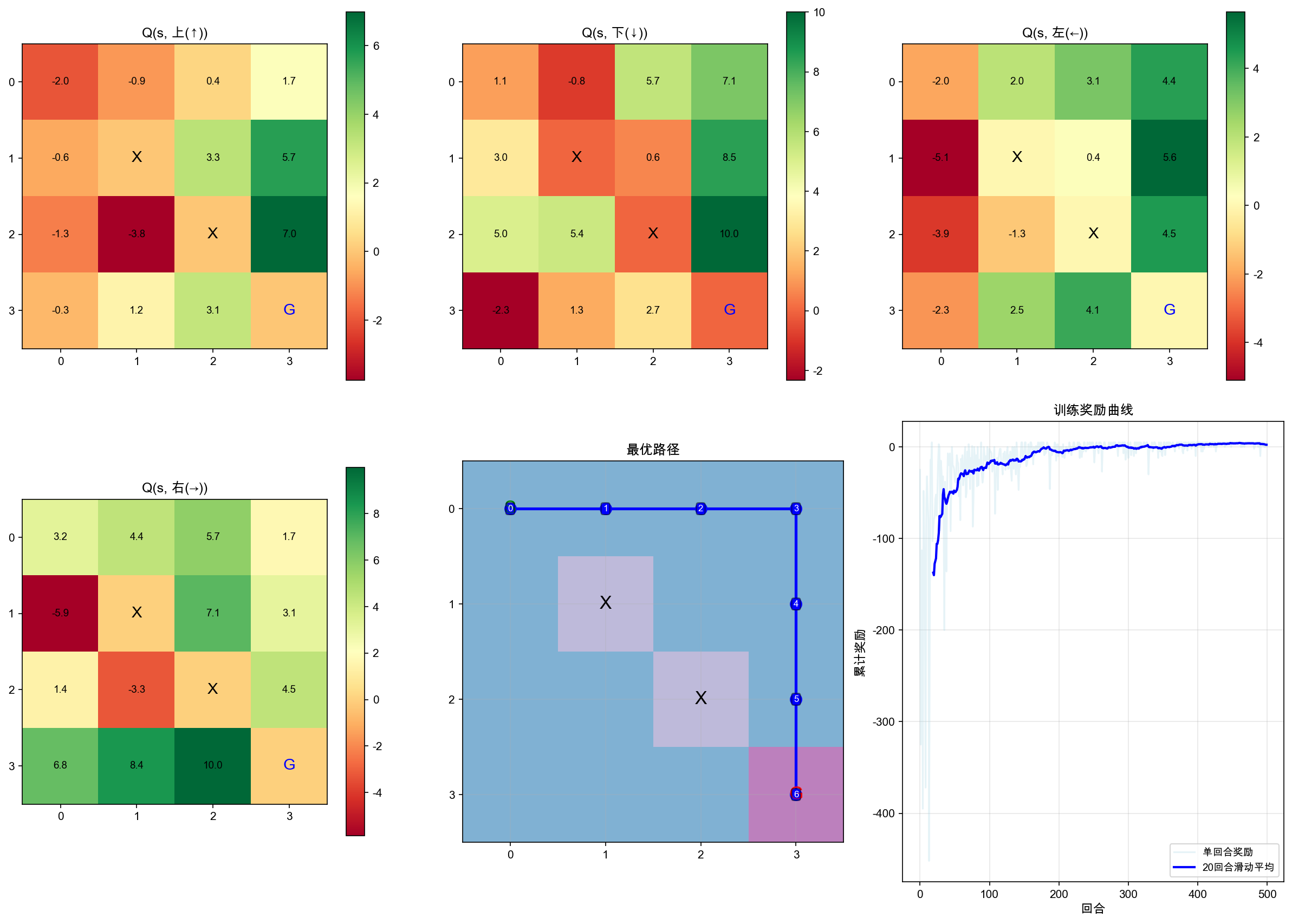
def visualize_results(Q, episode_rewards, env):
    """
    可视化 Q-Learning 的学习结果
    - 图1:每个动作的 Q 值热力图
    - 图2:最优路径在网格上的展示
    - 图3:每回合累计奖励的变化曲线
    """
    plt.rcParams['font.sans-serif'] = ['Arial Unicode MS', 'SimHei']
    plt.rcParams['axes.unicode_minus'] = False

    fig = plt.figure(figsize=(16, 12))

    # ------------------------------------------
    # 图1:四个动作的 Q 值热力图
    # ------------------------------------------
    action_names_short = ['上(↑)', '下(↓)', '左(←)', '右(→)']

    for i in range(4):
        ax = fig.add_subplot(2, 3, i + 1)
        q_values = Q[:, :, i]  # 取出某个动作在所有状态的 Q 值

        im = ax.imshow(q_values, cmap='RdYlGn', aspect='equal')
        # 在每个格子上标注 Q 值
        for r in range(env.rows):
            for c in range(env.cols):
                if (r, c) in env.obstacles:
                    ax.text(c, r, 'X', ha='center', va='center',
                            fontsize=14, fontweight='bold', color='black')
                elif (r, c) == env.goal:
                    ax.text(c, r, 'G', ha='center', va='center',
                            fontsize=14, fontweight='bold', color='blue')
                else:
                    ax.text(c, r, f'{q_values[r, c]:.1f}', ha='center', va='center',
                            fontsize=9)
        ax.set_title(f'Q(s, {action_names_short[i]})', fontsize=12)
        ax.set_xticks(range(env.cols))
        ax.set_yticks(range(env.rows))
        ax.set_xticklabels(range(env.cols))
        ax.set_yticklabels(range(env.rows))
        plt.colorbar(im, ax=ax, shrink=0.8)

    # ------------------------------------------
    # 图2:最优路径可视化
    # ------------------------------------------
    ax_path = fig.add_subplot(2, 3, 5)
    # 绘制网格底色
    grid = np.zeros((env.rows, env.cols))
    for obs in env.obstacles:
        grid[obs] = -1
    grid[env.goal] = 2

    ax_path.imshow(grid, cmap='Set3', aspect='equal', vmin=-2, vmax=3)

    # 提取并绘制最优路径
    path = extract_optimal_path(Q, env)
    path_rows = [p[0] for p in path]
    path_cols = [p[1] for p in path]
    ax_path.plot(path_cols, path_rows, 'b-o', linewidth=2.5, markersize=10)

    # 标注起点、终点、障碍物
    ax_path.text(0, 0, 'S', ha='center', va='center', fontsize=16,
                 fontweight='bold', color='green')
    ax_path.text(3, 3, 'G', ha='center', va='center', fontsize=16,
                 fontweight='bold', color='red')
    for obs in env.obstacles:
        ax_path.text(obs[1], obs[0], 'X', ha='center', va='center',
                     fontsize=16, fontweight='bold', color='black')

    # 在路径上标注步数
    for idx, (r, c) in enumerate(path):
        ax_path.text(c, r, str(idx), ha='center', va='center',
                     fontsize=8, color='white',
                     bbox=dict(boxstyle='round,pad=0.2', fc='blue', alpha=0.5))

    ax_path.set_title('最优路径', fontsize=12)
    ax_path.set_xticks(range(env.cols))
    ax_path.set_yticks(range(env.rows))
    ax_path.set_xticklabels(range(env.cols))
    ax_path.set_yticklabels(range(env.rows))
    ax_path.grid(True, alpha=0.3)

    # ------------------------------------------
    # 图3:训练奖励曲线
    # ------------------------------------------
    ax_reward = fig.add_subplot(2, 3, 6)
    ax_reward.plot(episode_rewards, alpha=0.3, color='lightblue', label='单回合奖励')
    # 计算滑动平均
    window = 20
    if len(episode_rewards) >= window:
        moving_avg = np.convolve(episode_rewards,
                                 np.ones(window) / window, mode='valid')
        ax_reward.plot(range(window - 1, len(episode_rewards)),
                       moving_avg, color='blue', linewidth=2,
                       label=f'{window}回合滑动平均')
    ax_reward.set_xlabel('回合', fontsize=11)
    ax_reward.set_ylabel('累计奖励', fontsize=11)
    ax_reward.set_title('训练奖励曲线', fontsize=12)
    ax_reward.legend(fontsize=9)
    ax_reward.grid(True, alpha=0.3)

    plt.tight_layout()
    plt.savefig('output/gridworld_q_learning_results.png', dpi=150, bbox_inches='tight')
    print("\n图表已保存至 output/gridworld_q_learning_results.png")
    plt.show()


# ==========================================
# 第四部分:主程序
# ==========================================
def main():
    """主函数:创建环境 → 训练 → 打印 Q 表 → 可视化"""

    # 创建 GridWorld 环境
    env = GridWorld()
    print("GridWorld 环境创建完成")
    print(f"  起点: {env.start}")
    print(f"  终点: {env.goal}")
    print(f"  障碍物: {env.obstacles}")
    print(f"  动作空间: {env.action_names}")

    # 训练 Q-Learning
    Q, episode_rewards, episode_steps = train_q_learning(env, n_episodes=500)

    # 打印最终 Q 表
    print_q_table(Q, env)

    # 提取并打印最优路径
    path = extract_optimal_path(Q, env)
    print(f"\n最优路径: {' → '.join([str(p) for p in path])}")
    print(f"路径长度: {len(path) - 1} 步")

    # 计算最优路径的总奖励
    total_r = 0
    for i in range(len(path) - 1):
        if i < len(path) - 2:
            total_r += -1  # 普通步骤:-1
        else:
            total_r += 10  # 到达终点的最后一步:+10
    print(f"最优路径总奖励: {total_r}")

    # 可视化结果
    visualize_results(Q, episode_rewards, env)


if __name__ == "__main__":
    main()
python
GridWorld 环境创建完成
  起点: (0, 0)
  终点: (3, 3)
  障碍物: [(1, 1), (2, 2)]
  动作空间: ['上(↑)', '下(↓)', '左(←)', '右(→)']
============================================================
  Q-Learning 训练
============================================================
  学习率 α = 0.1
  折扣因子 γ = 0.95
  初始探索率 ε = 1.0
  训练回合数 = 500
------------------------------------------------------------
  回合  100 | 近100回合平均奖励:  -53.89 | 平均步数:  26.4 | ε: 0.6058
  回合  200 | 近100回合平均奖励:   -9.74 | 平均步数:  11.1 | ε: 0.3670
  回合  300 | 近100回合平均奖励:   -0.70 | 平均步数:   7.9 | ε: 0.2223
  回合  400 | 近100回合平均奖励:    0.67 | 平均步数:   7.6 | ε: 0.1347
  回合  500 | 近100回合平均奖励:    3.44 | 平均步数:   6.6 | ε: 0.0816
------------------------------------------------------------

============================================================
  最终 Q 表
============================================================
状态        上(↑)        下(↓)        左(←)        右(→)        最优动作
------------------------------------------------------------
(0,0)          -2.01       1.09      -1.99       3.21     右(→)
(0,1)          -0.86      -0.84       1.97       4.44     右(→)
(0,2)           0.35       5.66       3.14       5.72     右(→)
(0,3)           1.68       7.07       4.37       1.70     下(↓)
(1,0)          -0.59       2.98      -5.10      -5.86     下(↓)
(1,1) 障碍      ---      ---      ---      ---     障碍物
(1,2)           3.32       0.64       0.35       7.07     右(→)
(1,3)           5.70       8.50       5.64       3.05     下(↓)
(2,0)          -1.31       5.02      -3.85       1.42     下(↓)
(2,1)          -3.76       5.40      -1.29      -3.26     下(↓)
(2,2) 障碍      ---      ---      ---      ---     障碍物
(2,3)           6.98      10.00       4.49       4.47     下(↓)
(3,0)          -0.32      -2.33      -2.27       6.82     右(→)
(3,1)           1.22       1.35       2.55       8.43     右(→)
(3,2)           3.13       2.69       4.10       9.99     右(→)
(3,3) 终点      ---      ---      ---      ---     终点
------------------------------------------------------------

最优路径: (0, 0) → (0, 1) → (0, 2) → (0, 3) → (1, 3) → (2, 3) → (3, 3)
路径长度: 6 步
最优路径总奖励: 5

图表已保存至 output/gridworld_q_learning_results.png