矿物识别系统实战------六种填充方法×六种模型全面对比
- 简介
- 一、训练前准备
- [二、逻辑回归(Logistic Regression)](#二、逻辑回归(Logistic Regression))
- [三、随机森林(Random Forest)](#三、随机森林(Random Forest))
- 四、支持向量机(SVM)
- 五、AdaBoost
- 六、XGBoost
- 七、高斯朴素贝叶斯(GaussianNB)
- 八、保存所有模型结果
- 总结
- 一、各填充方法下的模型表现汇总
-
- [1. 均值填充](#1. 均值填充)
- [2. 中位数填充](#2. 中位数填充)
- [3. 众数填充](#3. 众数填充)
- [4. 空值删除(CCA)](#4. 空值删除(CCA))
- [5. 线性回归填充](#5. 线性回归填充)
- [6. 随机森林填充](#6. 随机森林填充)
- 二、综合分析
简介
在上一篇博客当中我们对数据集进行处理,使用了6种方法进行数据填充,经过一系列操作得到可以直接放到模型里面训练的数据集。接下来我们将使用6种机器学习算法进行训练和预测。
【机器学习】矿物识别系统实战------从数据清洗到多模型对比
一、训练前准备
读取训练数据与测试数据
python
import pandas as pd

train_data = pd.read_excel(r"训练集数据(平均数).xlsx")
test_data = pd.read_excel(r"测试集数据(平均数).xlsx")

划分特征与标签
python
# 训练集:第1列为标签,其余为特征
train_data_x = train_data.iloc[:, 1:]   # 特征
train_data_y = train_data.iloc[:, 0]    # 标签

# 测试集:同样方式划分
test_data_x = test_data.iloc[:, 1:]     # 特征
test_data_y = test_data.iloc[:, 0]      # 标签
创建结果存储字典
python
result_data = {}   # 用于存储所有模型的评估结果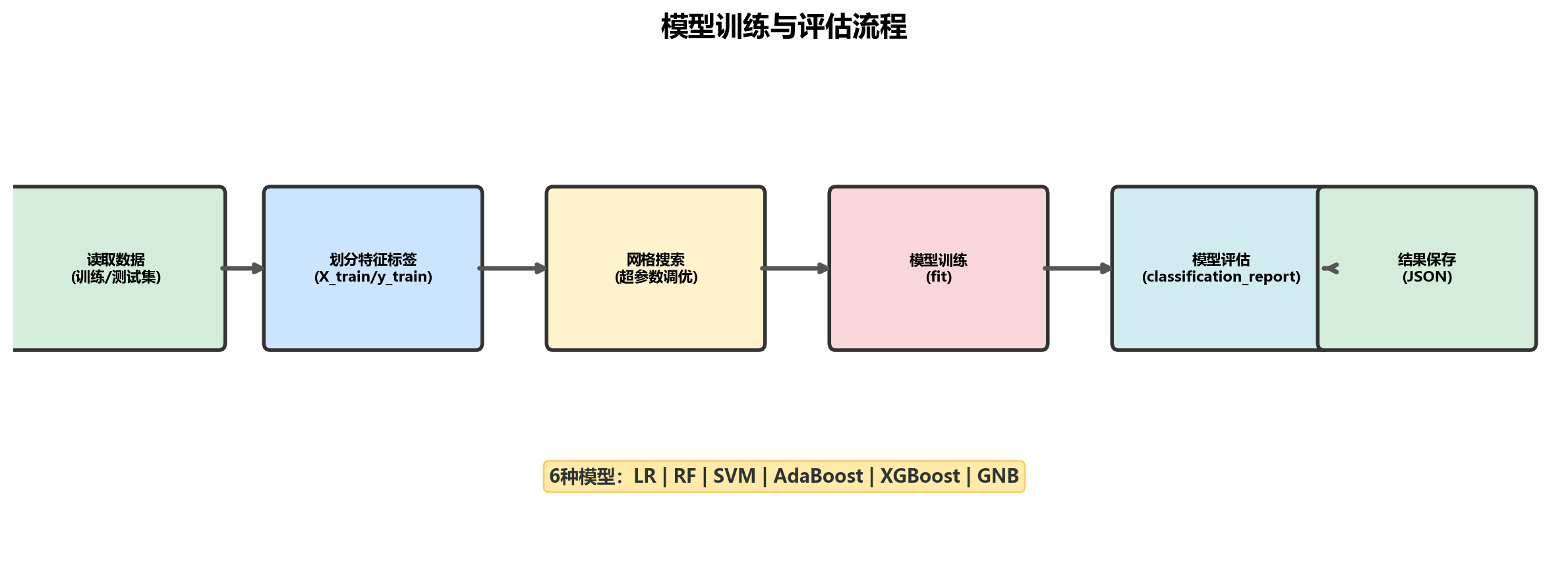
二、逻辑回归(Logistic Regression)
网格搜索调参
python
from sklearn.linear_model import LogisticRegression
from sklearn.model_selection import GridSearchCV

param_grid = {
    'penalty': ['l1', 'l2', 'elasticnet', 'none'],
    'C': [0.001, 0.01, 0.1, 1, 10, 100],
    'solver': ['newton-cg', 'lbfgs', 'liblinear', 'sag', 'saga'],
    'max_iter': [100, 200, 500],
    'multi_class': ['multinomial']
}

logreg = LogisticRegression()
grid_search = GridSearchCV(logreg, param_grid, cv=5)
grid_search.fit(train_data_x, train_data_y)
print("最佳参数:", grid_search.best_params_)
模型训练
python
LR_result = {}
lr = LogisticRegression(
    C=0.001,
    max_iter=100,
    penalty='none',
    solver='lbfgs'
)
lr.fit(train_data_x, train_data_y)
模型评估
python
from sklearn import metrics

# 训练集评估
train_predicted = lr.predict(train_data_x)
print('LR训练集表现:\n', metrics.classification_report(train_data_y, train_predicted))

# 测试集评估
test_predicted = lr.predict(test_data_x)
print('LR测试集表现:\n', metrics.classification_report(test_data_y, test_predicted))
结果提取
python
# 提取各类别召回率和整体准确率
report = metrics.classification_report(test_data_y, test_predicted, digits=6)
parts = report.split()

LR_result['recall_0'] = float(parts[6])
LR_result['recall_1'] = float(parts[11])
LR_result['recall_2'] = float(parts[16])
LR_result['recall_3'] = float(parts[21])
LR_result['acc'] = float(parts[25])

result_data['LR'] = LR_result
三、随机森林(Random Forest)
网格搜索调参
python
from sklearn.ensemble import RandomForestClassifier

param_grid = {
    'n_estimators': [50, 100, 200, 300],
    'max_depth': [None, 10, 20, 30, 40],
    'min_samples_split': [2, 5, 10],
    'min_samples_leaf': [1, 2, 4],
    'max_features': ['sqrt', 'log2', None],
    'bootstrap': [True, False],
    'criterion': ['gini', 'entropy']
}

rf_model = RandomForestClassifier()
grid_search = GridSearchCV(rf_model, param_grid, cv=5)
grid_search.fit(train_data_x, train_data_y)
print("最佳参数:", grid_search.best_params_)
模型训练
python
RF_result = {}
rf = RandomForestClassifier(
    bootstrap=False,
    max_depth=20,
    max_features='log2',
    min_samples_leaf=1,
    min_samples_split=2,
    n_estimators=50,
    random_state=487
)
rf.fit(train_data_x, train_data_y)
模型评估
python
# 训练集评估
train_predicted = rf.predict(train_data_x)
print('RF训练集表现:\n', metrics.classification_report(train_data_y, train_predicted))

# 测试集评估
test_predicted = rf.predict(test_data_x)
print('RF测试集表现:\n', metrics.classification_report(test_data_y, test_predicted))
结果提取
python
report = metrics.classification_report(test_data_y, test_predicted, digits=6)
parts = report.split()

RF_result['recall_0'] = float(parts[6])
RF_result['recall_1'] = float(parts[11])
RF_result['recall_2'] = float(parts[16])
RF_result['recall_3'] = float(parts[21])
RF_result['acc'] = float(parts[25])

result_data['RF'] = RF_result
四、支持向量机(SVM)
网格搜索调参
python
from sklearn.svm import SVC

param_grid = {
    'C': [0.001, 0.01, 0.1, 1, 2],
    'kernel': ['linear', 'poly', 'rbf', 'sigmoid'],
    'gamma': ['scale', 'auto', 0.001, 0.01, 0.1, 1],
    'degree': [2, 3, 4],
    'coef0': [0.0, 0.1, 1.0],
    'shrinking': [True, False],
    'probability': [False, True],
    'class_weight': [None, 'balanced']
}

svm_model = SVC()
grid_search = GridSearchCV(svm_model, param_grid, cv=5)
grid_search.fit(train_data_x, train_data_y)
print("最佳参数:", grid_search.best_params_)
模型训练
python
SVM_result = {}
svm = SVC(
    C=1,
    coef0=0.1,
    degree=4,
    gamma=1,
    kernel='poly',
    probability=True,
    random_state=100
)
svm.fit(train_data_x, train_data_y)
模型评估与结果提取
python
# 测试集评估
test_predicted = svm.predict(test_data_x)
print('SVM测试集表现:\n', metrics.classification_report(test_data_y, test_predicted))

report = metrics.classification_report(test_data_y, test_predicted, digits=6)
parts = report.split()

SVM_result['recall_0'] = float(parts[6])
SVM_result['recall_1'] = float(parts[11])
SVM_result['recall_2'] = float(parts[16])
SVM_result['recall_3'] = float(parts[21])
SVM_result['acc'] = float(parts[25])

result_data['SVM'] = SVM_result
五、AdaBoost
网格搜索调参
python
from sklearn.ensemble import AdaBoostClassifier
from sklearn.tree import DecisionTreeClassifier

param_grid = {
    'n_estimators': [50, 100, 200, 300],
    'learning_rate': [0.01, 0.1, 0.5, 1.0, 1.5],
    'algorithm': ['SAMME', 'SAMME.R'],
    'base_estimator__max_depth': [1, 2, 3, 4],
    'base_estimator__min_samples_split': [2, 5],
    'base_estimator__min_samples_leaf': [1, 2]
}

ada_model = AdaBoostClassifier()
grid_search = GridSearchCV(ada_model, param_grid, cv=5)
grid_search.fit(train_data_x, train_data_y)
print("最佳参数:", grid_search.best_params_)
模型训练
python
AdaBoost_result = {}
ada = AdaBoostClassifier(
    algorithm='SAMME',
    base_estimator=DecisionTreeClassifier(max_depth=2),
    n_estimators=200,
    learning_rate=1.0,
    random_state=0
)
ada.fit(train_data_x, train_data_y)
模型评估与结果提取
python
test_predicted = ada.predict(test_data_x)
print('AdaBoost测试集表现:\n', metrics.classification_report(test_data_y, test_predicted))

report = metrics.classification_report(test_data_y, test_predicted, digits=6)
parts = report.split()

AdaBoost_result['recall_0'] = float(parts[6])
AdaBoost_result['recall_1'] = float(parts[11])
AdaBoost_result['recall_2'] = float(parts[16])
AdaBoost_result['recall_3'] = float(parts[21])
AdaBoost_result['acc'] = float(parts[25])

result_data['AdaBoost'] = AdaBoost_result
六、XGBoost
网格搜索调参
python
import xgboost as xgb

param_grid = {
    'learning_rate': [0.01, 0.05, 0.1, 0.2],
    'n_estimators': [100, 200, 300, 500],
    'max_depth': [3, 5, 7, 9],
    'min_child_weight': [1, 3, 5],
    'subsample': [0.6, 0.8, 1.0],
    'colsample_bytree': [0.6, 0.8, 1.0],
    'gamma': [0, 0.1, 0.2]
}

xgb_model = xgb.XGBClassifier(objective='multi:softmax', num_class=5, seed=0)
grid_search = GridSearchCV(xgb_model, param_grid, cv=5)
grid_search.fit(train_data_x, train_data_y)
print("最佳参数:", grid_search.best_params_)
模型训练
python
XGBoost_result = {}
xgb_model = xgb.XGBClassifier(
    learning_rate=0.05,
    n_estimators=200,
    num_class=5,
    max_depth=7,
    min_child_weight=1,
    gamma=0,
    subsample=0.6,
    colsample_bytree=0.8,
    objective='multi:softmax',
    seed=0
)
xgb_model.fit(train_data_x, train_data_y)
模型评估与结果提取
python
test_predicted = xgb_model.predict(test_data_x)
print('XGBoost测试集表现:\n', metrics.classification_report(test_data_y, test_predicted))

report = metrics.classification_report(test_data_y, test_predicted, digits=6)
parts = report.split()

XGBoost_result['recall_0'] = float(parts[6])
XGBoost_result['recall_1'] = float(parts[11])
XGBoost_result['recall_2'] = float(parts[16])
XGBoost_result['recall_3'] = float(parts[21])
XGBoost_result['acc'] = float(parts[25])

result_data['XGBoost'] = XGBoost_result
七、高斯朴素贝叶斯(GaussianNB)
模型训练
python
from sklearn.naive_bayes import GaussianNB

GNB_result = {}
gnb = GaussianNB()
gnb.fit(train_data_x, train_data_y)
模型评估与结果提取
python
test_predicted = gnb.predict(test_data_x)
print('GNB测试集表现:\n', metrics.classification_report(test_data_y, test_predicted))

report = metrics.classification_report(test_data_y, test_predicted, digits=6)
parts = report.split()

GNB_result['recall_0'] = float(parts[6])
GNB_result['recall_1'] = float(parts[11])
GNB_result['recall_2'] = float(parts[16])
GNB_result['recall_3'] = float(parts[21])
GNB_result['acc'] = float(parts[25])

result_data['GNB'] = GNB_result
八、保存所有模型结果
python
import json

final_result = {}
final_result['mean_fill'] = result_data

with open('平均值填充result.json', 'w', encoding='utf-8') as f:
    json.dump(final_result, f, ensure_ascii=False, indent=4)
总结
六种模型性能对比
| 维度 | 内容 |
|---|---|
| 填充方法 | 均值填充、中位数填充、众数填充、空值删除、线性回归填充、随机森林填充 |
| 机器学习模型 | LR(逻辑回归)、RF(随机森林)、SVM、AdaBoost、GNB(高斯朴素贝叶斯)、XGBoost |
| 评估指标 | 各类别召回率(recall_0~3)、整体准确率(acc) |
一、各填充方法下的模型表现汇总
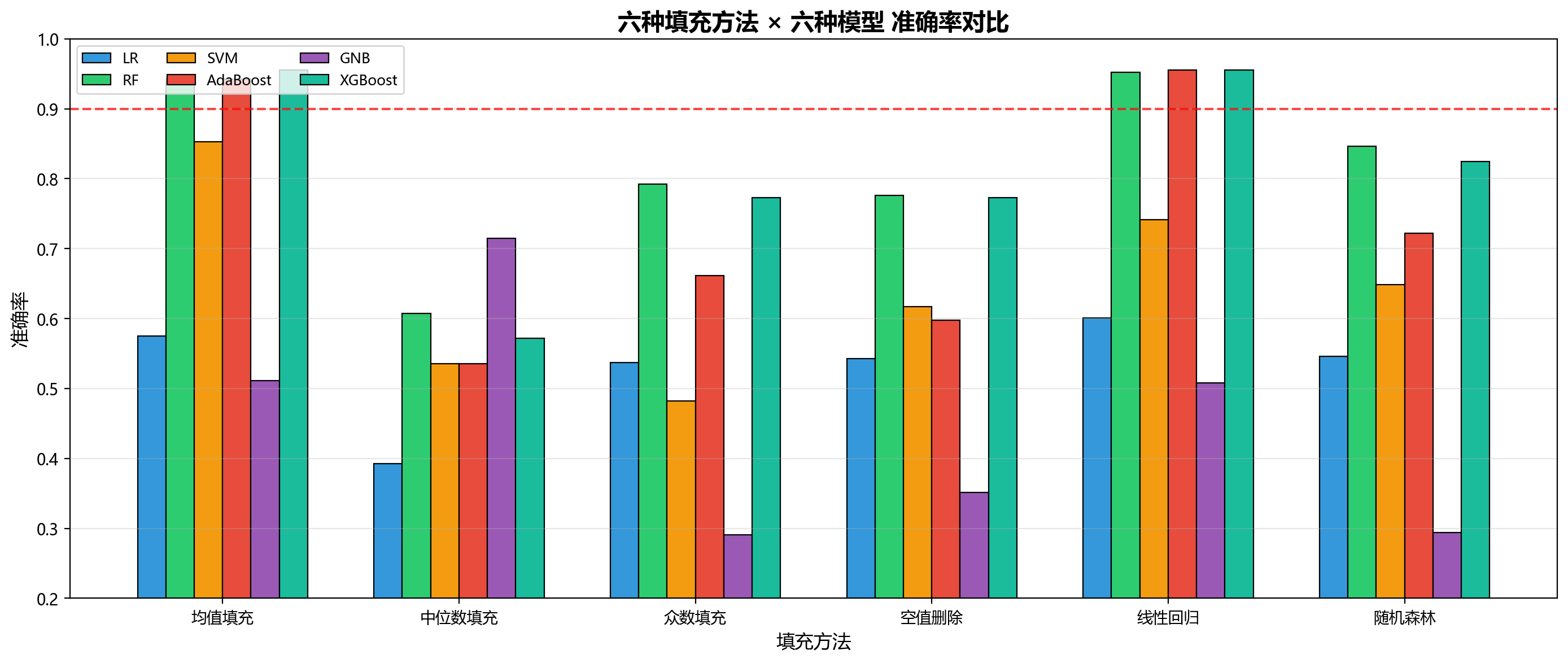
1. 均值填充
| 模型 | recall_0 | recall_1 | recall_2 | recall_3 | acc |
|---|---|---|---|---|---|
| LR | 0.8373 | 0.0297 | 0.9000 | 0.6875 | 0.5751 |
| RF | 0.9699 | 0.9307 | 0.9667 | 0.6875 | 0.9425 |
| SVM | 0.9518 | 0.7624 | 0.8667 | 0.3750 | 0.8530 |
| AdaBoost | 0.9639 | 0.9505 | 1.0000 | 0.5625 | 0.9425 |
| GNB | 0.7289 | 0.0198 | 0.8333 | 0.7500 | 0.5112 |
| XGBoost | 0.9819 | 0.9406 | 0.9667 | 0.7500 | 0.9553 |
均值填充下最优模型:XGBoost(acc=0.9553)
2. 中位数填充
| 模型 | recall_0 | recall_1 | recall_2 | recall_3 | acc |
|---|---|---|---|---|---|
| LR | 0.5455 | 0.1667 | 1.0000 | 0.3333 | 0.3929 |
| RF | 0.7273 | 0.5833 | 0.0000 | 0.6667 | 0.6071 |
| SVM | 0.6364 | 0.5833 | 0.0000 | 0.3333 | 0.5357 |
| AdaBoost | 0.6364 | 0.5833 | 0.0000 | 0.3333 | 0.5357 |
| GNB | 0.7273 | 0.8333 | 0.0000 | 0.6667 | 0.7143 |
| XGBoost | 0.5455 | 0.5833 | 0.5000 | 0.6667 | 0.5714 |
中位数填充下最优模型:GNB(acc=0.7143)
3. 众数填充
| 模型 | recall_0 | recall_1 | recall_2 | recall_3 | acc |
|---|---|---|---|---|---|
| LR | 0.8133 | 0.1386 | 0.3000 | 0.6250 | 0.5367 |
| RF | 0.9036 | 0.7525 | 0.5000 | 0.4375 | 0.7923 |
| SVM | 0.8072 | 0.0000 | 0.0667 | 0.9375 | 0.4824 |
| AdaBoost | 0.7771 | 0.6337 | 0.2333 | 0.4375 | 0.6613 |
| GNB | 0.4217 | 0.0198 | 0.2000 | 0.8125 | 0.2907 |
| XGBoost | 0.8675 | 0.7525 | 0.5333 | 0.3750 | 0.7732 |
众数填充下最优模型:RF(acc=0.7923)
4. 空值删除(CCA)
| 模型 | recall_0 | recall_1 | recall_2 | recall_3 | acc |
|---|---|---|---|---|---|
| LR | 0.8193 | 0.1386 | 0.4000 | 0.5000 | 0.5431 |
| RF | 0.8855 | 0.7525 | 0.4333 | 0.4375 | 0.7764 |
| SVM | 0.7892 | 0.2970 | 0.6000 | 0.8750 | 0.6166 |
| AdaBoost | 0.6807 | 0.5644 | 0.3667 | 0.3750 | 0.5974 |
| GNB | 0.5542 | 0.0198 | 0.1333 | 0.7500 | 0.3514 |
| XGBoost | 0.8795 | 0.7228 | 0.5333 | 0.4375 | 0.7732 |
空值删除下最优模型:RF(acc=0.7764)
5. 线性回归填充
| 模型 | recall_0 | recall_1 | recall_2 | recall_3 | acc |
|---|---|---|---|---|---|
| LR | 0.8494 | 0.0594 | 0.9333 | 0.8125 | 0.6006 |
| RF | 0.9759 | 0.9307 | 0.9667 | 0.8125 | 0.9521 |
| SVM | 0.8795 | 0.4455 | 0.9667 | 0.7500 | 0.7412 |
| AdaBoost | 0.9699 | 0.9604 | 0.9667 | 0.7500 | 0.9553 |
| GNB | 0.7289 | 0.0198 | 0.8000 | 0.7500 | 0.5080 |
| XGBoost | 0.9759 | 0.9604 | 0.9667 | 0.6875 | 0.9553 |
线性回归填充下最优模型:AdaBoost 和 XGBoost(acc=0.9553)
6. 随机森林填充
| 模型 | recall_0 | recall_1 | recall_2 | recall_3 | acc |
|---|---|---|---|---|---|
| LR | 0.8373 | 0.0891 | 0.4667 | 0.5625 | 0.5463 |
| RF | 0.9036 | 0.8119 | 0.6000 | 0.9375 | 0.8466 |
| SVM | 0.7771 | 0.3366 | 0.8000 | 1.0000 | 0.6486 |
| AdaBoost | 0.7229 | 0.7624 | 0.5667 | 0.7500 | 0.7220 |
| GNB | 0.4337 | 0.0198 | 0.2000 | 0.7500 | 0.2939 |
| XGBoost | 0.8675 | 0.8119 | 0.6333 | 0.8125 | 0.8243 |
随机森林填充下最优模型:XGBoost(acc=0.8243)
二、综合分析
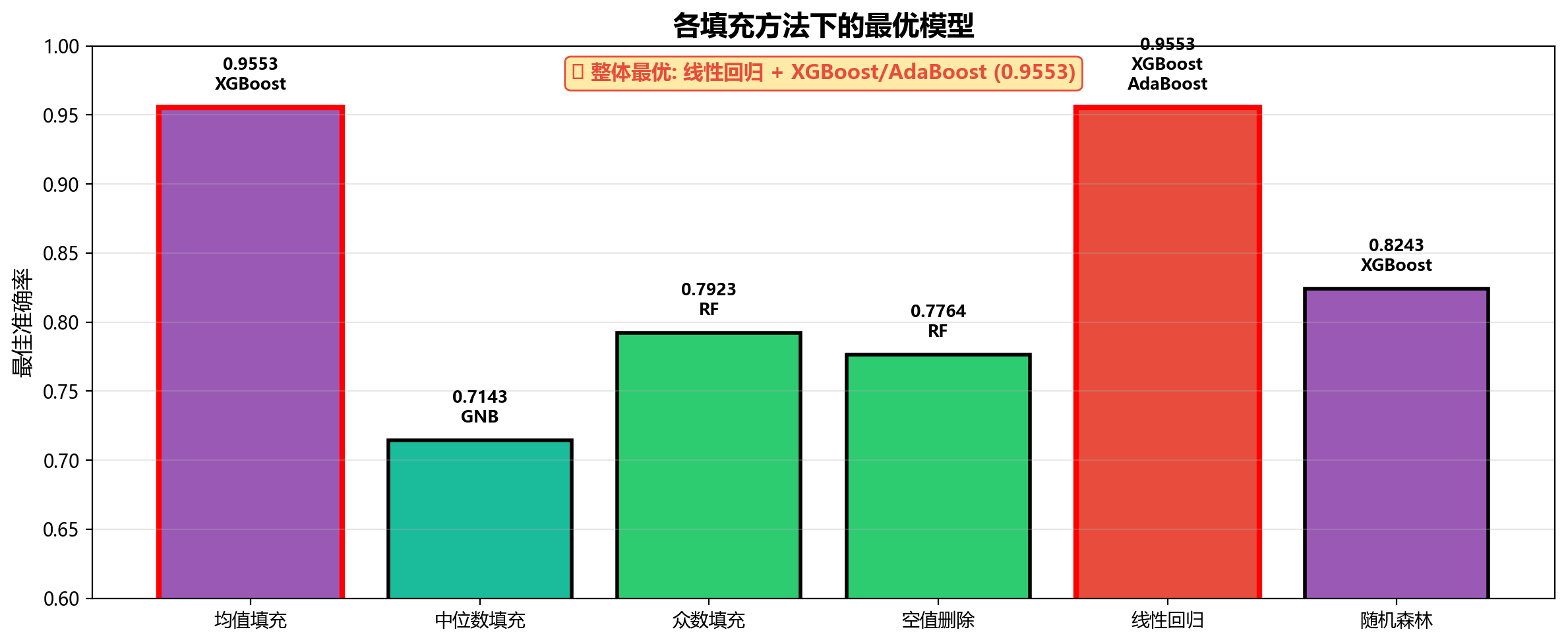
1. 各填充方法下最优模型汇总
| 填充方法 | 最优模型 | 最佳准确率 |
|---|---|---|
| 均值填充 | XGBoost | 0.9553 |
| 中位数填充 | GNB | 0.7143 |
| 众数填充 | RF | 0.7923 |
| 空值删除 | RF | 0.7764 |
| 线性回归填充 | AdaBoost / XGBoost | 0.9553 |
| 随机森林填充 | XGBoost | 0.8243 |
2. 关键发现
整体最优组合
线性回归填充 + XGBoost / AdaBoost(准确率 0.9553)
模型表现分析
| 模型 | 最佳表现场景 | 最佳准确率 | 特点 |
|---|---|---|---|
| XGBoost | 均值填充、线性回归填充 | 0.9553 | 在多种填充方法下表现稳定且最优 |
| RF | 众数填充、空值删除 | 0.7923 | 集成学习优势明显 |
| AdaBoost | 线性回归填充 | 0.9553 | 与XGBoost并列最优 |
| GNB | 中位数填充 | 0.7143 | 简单模型在特定场景下表现突出 |
| SVM | 均值填充 | 0.8530 | 核方法有效但调参复杂 |
| LR | --- | 0.6006 | 线性模型表达能力有限 |
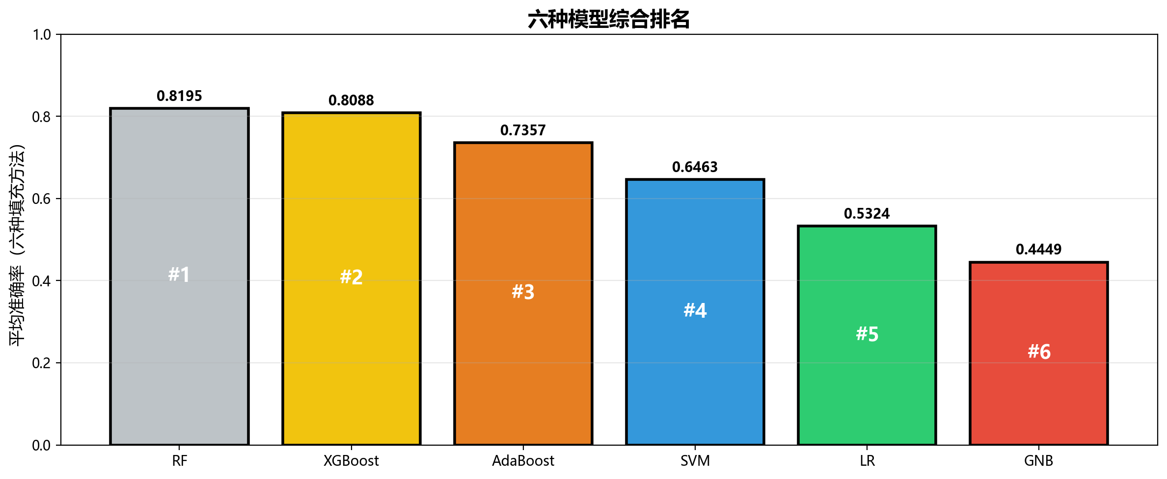
3. 结论
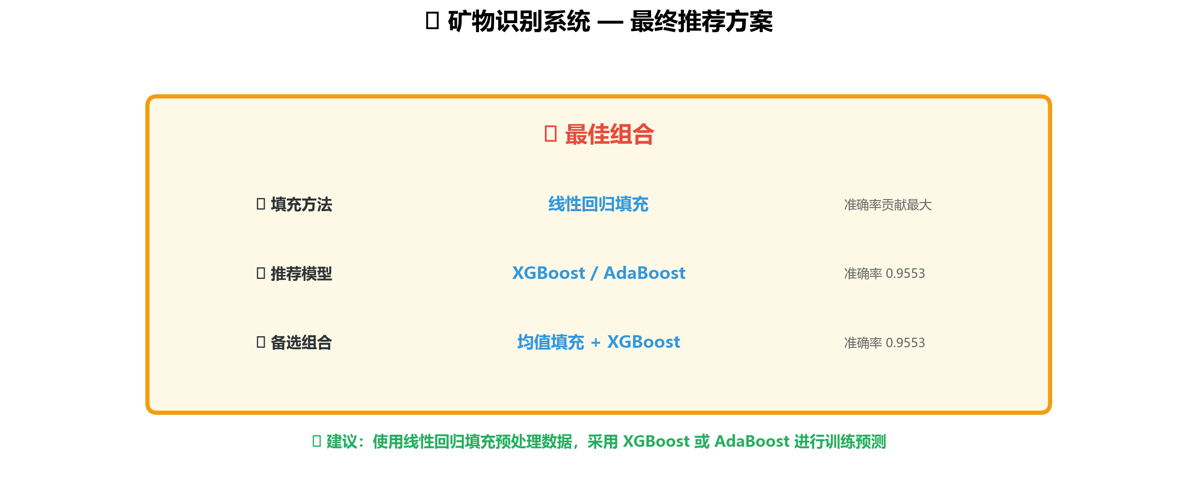
- 最优填充方法 :线性回归填充 和均值填充效果最佳,准确率均达到 0.955
- 最优模型 :XGBoost 在多种填充方法下表现稳定,是最值得推荐的模型
- 推荐组合 :线性回归填充 + XGBoost,准确率 0.9553