PyTorch计算机视觉（5）——生成对抗网络（Generative Adversarial Network，GAN）

PyTorch计算机视觉（5）------生成对抗网络（Generative Adversarial Network，GAN）

• • [0. 前言](#0. 前言)
  • [1. 生成对抗网络理论基础](#1. 生成对抗网络理论基础)
  • [2. 实现生成对抗网络](#2. 实现生成对抗网络)
  • [3. 实现生成对抗网络生成 MNIST 图像](#3. 实现生成对抗网络生成 MNIST 图像)
  • 小结
  • 系列链接

0. 前言

图像生成任务不论对人类还是计算机而言，都比图像分类更具挑战性。自生成对抗网络提出以来，众多基于生成对抗网络 (Generative Adversarial Network, GAN) 的算法相继涌现。如今，计算机已能通过学习生成以假乱真的人脸图像。GAN 架构包含两个神经网络：生成器与判别器。生成器负责从纯噪声中合成模拟数据样本，而判别器则通过对比真实样本与生成样本进行真伪判别。在模型训练过程中，两个网络相互博弈：生成器持续提升伪造能力以迷惑判别器，判别器则不断优化其鉴伪能力。

当训练达到平衡时，生成器创造的数据将逼真到令判别器无法甄别真伪的程度。此时 GAN 已学习到数据集中图像像素的概率分布函数 (probability distribution function, PDF)，计算机可基于该分布的参数生成与真实图像高度相似的伪造图像。

1. 生成对抗网络理论基础

生成对抗网络 (Generative Adversarial Network, GAN) 中的生成器 (G) 负责将一维噪声向量转换为伪造图像。噪声向量中的元素个数可以是 1、2，甚至超过 100，这些向量通常取自标准正态分布。生成器包含大量待训练参数 ( θ g θ_g θg)。

判别器 (D) 则被训练用于区分数据集中的真实图像与生成图像，其本身也拥有待训练参数 ( θ d θ_d θd)。这一过程可类比艺术教学：生成器如同学徒，判别器宛若严师。学徒通过观摩大师真迹进行临摹，教师则持续指出画作缺陷并提供改进建议。经过多次迭代，学徒最终能创作出以假乱真的摹本------这是理想的训练结果。但若学徒悟性不足，或教师专业欠缺，训练便可能以失败告终。

生成对抗网络的模型训练至今仍具挑战性，其中一个核心难题是"模式坍塌"现象。例如，耗费 120 分钟训练生成 MNIST 手写数字的模型后，可能发现输出仅包含单一数字。两个模型中含有大量参数，代码中还存在诸多超参数，如何快速调整这些参数以达到预期效果？在应对这些训练挑战之前，我们首先需要构建 GAN 的训练框架。该框架包含四个组成部分：数据输入模块、双模型构建模块、模型训练模块和数据可视化模块。判别器模型 D 和生成器模型 G 的训练通过以下循环流程实现(设数据加载器批大小为 m)：

1. 从数据加载器获取真实图像批次： { x 1 , x 2 , . . . , x m } \{x_1, x_2,..., x_m\} {x1,x2,...,xm}

2. 使用模型 D 将 x i x_i xi 转换为标量 y ^ i = D ( x i ) ∈ 0 , 1 , ( i = 1 , 2 , . . . , m ) \hat y_i = D(x_i)∈0,1,\ (i = 1, 2, ..., m) y^i=D(xi)∈0,1, (i=1,2,...,m)

3. 设置所有真实图像的目标标签为 1： y i = 1 , ( i = 1 , 2 , . . . , m ) y_i = 1,\ (i = 1, 2, ..., m) yi=1, (i=1,2,...,m)

4. 计算目标值与预测值之间的二元交叉熵损失： 1 m ∑ i = 1 m ln ⁡ ( D ( x i ) ) \frac{1}{m} \sum_{i=1}^{m} \ln(D(x_i)) m1∑i=1mln(D(xi))

5. 从标准正态分布生成一个噪声向量批次： { z 1 , z 2 , . . . , z m } \{z_1, z_2, ..., z_m\} {z1,z2,...,zm}

6. 通过生成器生成伪造图像批次： x ~ i = G ( z i ) , ( i = 1 , 2 , . . . , m ) \tilde x_i = G(z_i),\ (i = 1, 2, ..., m) x~i=G(zi), (i=1,2,...,m)

7. 将伪造图像转换为标量 D ( x ~ i ) ∈ 0 , 1 D(\tilde x_i)∈0,1 D(x~i)∈0,1 作为伪造样本预测

8. 设置所有伪造图像的目标标签为 0

9. 计算不更新模型 G 时的 BCE 损失： − 1 m ∑ i = 1 m l n ( 1 − D ( x ~ i ) ) -\frac 1m∑_{i=1}^mln(1-D(\tilde x_i)) −m1∑i=1mln(1−D(x~i))

10. 计算模型 D 的损失：

    L D ( θ d ) = − 1 m ∑ i = 1 m l n ( D ( x i ) ) − 1 m ∑ i = 1 m ( 1 − l n ( D ( x ~ i ) ) ) L D ( θ d ) = − E l n ( D ( X ) ) − E l n ( 1 − D ( G ( Z ) ) ) → − ∫ p r ( x ) l n D ( X ) d x − ∫ p z ( z ) l n 1 − D ( G ( z ) ) d z → − ∫ p r ( x ) l n D ( X ) d x − ∫ p g ( x ) l n 1 − D ( x ) d x = − ∫ ( p r ( x ) l n D ( x ) + p g ( x ) l n 1 − D ( x ) ) d x L_D(\theta_d)=-\frac 1m\sum_{i=1}^mln(D(x_i))-\frac 1m\sum_{i=1}^m(1-ln(D(\tilde x_i)))\\ L_D(\theta_d)=-Eln(D(X))-Eln(1-D(G(Z)))\\ \rightarrow -\int p_r(x)lnD(X)dx-\int p_z(z)ln1-D(G(z))dz\\ \rightarrow -\int p_r(x)lnD(X)dx-\int p_g(x)ln1-D(x)dx\\ =-\int(p_r(x)lnD(x)+p_g(x)ln1-D(x))dx LD(θd)=−m1i=1∑mln(D(xi))−m1i=1∑m(1−ln(D(x~i)))LD(θd)=−Eln(D(X))−Eln(1−D(G(Z)))→−∫pr(x)lnD(X)dx−∫pz(z)ln1−D(G(z))dz→−∫pr(x)lnD(X)dx−∫pg(x)ln1−D(x)dx=−∫(pr(x)lnD(x)+pg(x)ln1−D(x))dx

    在生成器 G 固定的前提下，我们可以通过令损失函数在给定 x x x 处的导数为零(即 d d D ( x ) ( p r ( x ) l n D ( X ) + p g ( x ) l n 1 − D ( x ) ) = 0 \frac {d}{dD(x)}(p_r(x)lnD(X)+p_g(x)ln1-D(x))=0 dD(x)d(pr(x)lnD(X)+pg(x)ln1−D(x))=0 )来求解最优判别器 D*，从而最小化损失函数。

    经推导得出最优判别器的表达式为： D G ∗ ( x ) = p r ( x ) p r ( x ) + p g ( x ) D^*_G(x) = \frac {p_r(x)}{p_r(x) + p_g(x)} DG∗(x)=pr(x)+pg(x)pr(x)，其中：

    L D ( θ d ) = 2 ln ⁡ ( 2 ) − 2 D J S ( p r ∥ p g ) L_D(\theta_d) = 2 \ln (2) - 2 D_{JS} (p_r \parallel p_g) LD(θd)=2ln(2)−2DJS(pr∥pg)

    根据：

    0 ≤ D J S ( p r ∥ p g ) ≤ ln ⁡ ( 2 ) 0 \leq D_{JS} (p_r \parallel p_g) \leq \ln (2) 0≤DJS(pr∥pg)≤ln(2)

    因此：

    0 ≤ L D ( θ d ) ≤ 2 ln ⁡ ( 2 ) 0 \leq L_D(\theta_d) \leq 2 \ln (2) 0≤LD(θd)≤2ln(2)

    当 p r = p g p_r = p_g pr=pg 时，模型 D 的损失达到最大值： 2 ln ⁡ ( 2 ) 2 \ln (2) 2ln(2)

11. 更新 D 的参数 θ d \theta_d θd，不改变 θ g \theta_g θg ：

    θ d ← θ d − η ∇ θ d L D ( θ d ) \theta_d \leftarrow \theta_d - \eta \nabla_{\theta_d} L_D(\theta_d) θd←θd−η∇θdLD(θd)

12. 从正态分布采样新噪声批次： { z 1 , z 2 , . . . , z m } \{z_1, z_2, ..., z_m\} {z1,z2,...,zm}

13. 使用噪声生成新伪造图像批次： x i = G ( z i ) x_i = G(z_i) xi=G(zi)

14. 将每个 x i x_i xi 转换为标量 D ( x i ) ∈ 0 , 1 D(x_i) \in 0, 1 D(xi)∈0,1 作为预测结果

15. 设置所有伪造图像目标标签为 1

16. 计算 BCE 损失：

    L G ( θ g ) = − 1 m ∑ i = 1 m l n ( D ( x ~ i ) ) L_G(\theta_g)=-\frac 1m\sum_{i=1}^mln(D(\tilde x_i)) LG(θg)=−m1i=1∑mln(D(x~i))

17. 使用 θ g ← θ g − η ∇ θ g L G ( θ g ) \theta_g \leftarrow \theta_g - \eta \nabla_{\theta_g} L_G(\theta_g) θg←θg−η∇θgLG(θg) 更新 G 的参数

2. 实现生成对抗网络

我们首先将生成对抗网络 (Generative Adversarial Network, GAN) 理论应用于一个简单数据集。接下来，生成器模型 (G) 和判别器模型 (D) 仅使用了两层全连接层(如下图所示)。这些模型处理三个空间的数据：

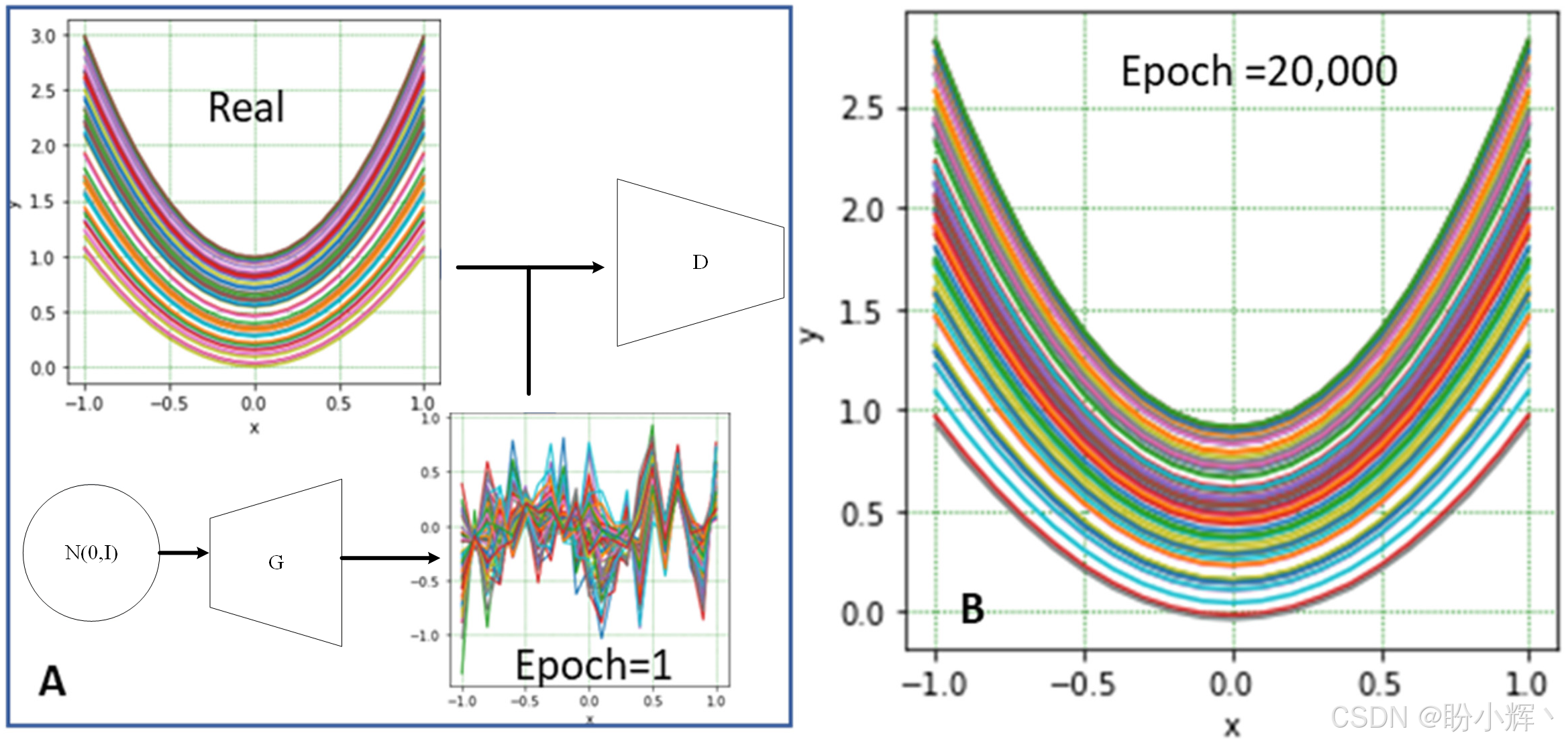
第一个是观测空间(即真实空间)，其中真实二次曲线数据具有 21 个维度。数据加载器中每批次的真实曲线数据来源于二次函数 y = a x 2 + b y = ax^2 + b y=ax2+b，其中 x x x 是通过 NumPy 函数 np.linspace(-1, 1, 21) 生成的一维数组。函数中的系数 a a a 通过均匀分布函数 np.random.uniform(1, 2, size=64) 生成并重塑为 64×1 的 NumPy 数组，常数项 b b b 设置为 ( a − 1 ) (a-1) (a−1)。函数 training_data() 生成的数据批次是一个 64 × 21 的数组。以下代码输出的图表展示了 64 条真实二次曲线。打印最后一条曲线 y[63] 的数据，我们将看到包含 21 个浮点数的一维 NumPy 数组。

import torch; import torch.nn as nn; import numpy as np; import pandas as pd
import matplotlib.pyplot as plt; from tqdm import trange
import torch.optim.lr_scheduler as lr_scheduler
n_epochs = 20000
batch_size = 64
z_dim = 2
n_hidden = 256
n_points = 21
n_batch = 5
lr = 1e-4
latent_noise = torch.randn(
    batch_size, z_dim, requires_grad=True, device='cuda')
x = np.linspace(-1, 1, n_points)
def training_data():
    a = np.random.uniform(1, 2, size=batch_size).reshape(-1,1)
    points = a*x*x + (a-1)
    return points
y = training_data()
def show_curves(x, y):
    fig, ax = plt.subplots(figsize=(4,4))
    for i in range(batch_size):
        ax.plot(x, y[i,:])
    ax.set(xlabel='x', ylabel='y', xticks=np.arange(-1.0, 1.1, 0.5))
    ax.grid(color='g', linestyle=':')
    plt.show()
show_curves(x,y)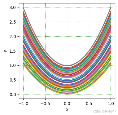

第二个是潜在空间，其维度设置为 2 (z_dim=2)，该空间中的噪声向量批次通过标准正态分布 N ( 0 , I ) N(0,I) N(0,I) 生成。名为 latent_noise 的噪声批次维度为 64×2。

第三个是由判别器模型 D 创建的临界空间，这是一个一维空间，其元素数量与批次大小一致。由于模型 D 的最终激活函数采用 Sigmoid 函数，临界空间中每个元素的取值区间为 [0,1]。当输入一批曲线数据(真实或生成)时，模型 D 会输出一组标量。执行代码 D(torch.cuda.FloatTensor(y)).T，将获得如下标量批次：

tensor([[0.5777, 0.5896, 0.5465, ..., 0.5571, 0.5436]], device='cuda:0', grad_fn=<PermuteBackward0>)

其中每个标量均对应一条真实图像的判别结果。

运行 D(G(latent_noise)).T，将得到另一组标量输出：

tensor([[0.5378, 0.5387, 0.5648, ..., 0.5702]], device='cuda:0', grad_fn=<PermuteBackward0>)

每个标量对应一条生成曲线。模型 D 将通过二元交叉熵损失函数进行训练，其目标是尽可能将真实曲线对应的标量提升至接近 1，同时将生成曲线对应的标量压制至接近 0。在模型 D 训练或参数更新过程中，生成器 G 的参数将保持冻结。随后，模型 G 将基于新采样的噪声向量，通过另一个二元交叉熵损失函数进行训练，该函数致力于将生成曲线的判别标量提升至接近 1。两个模型经过多次交替训练后，最终博弈结果将使得判别器对真实数据和生成数据的输出均趋近于 0.5，即 D(X) = D(G(Z)) = 0.5。

运行代码后，将观察到 64 条的二次曲线。变量 z_dim 表示二维噪声向量的维度，这些向量经过模型 G 的两层网络处理后，将生成包含 21 个点的伪造曲线。模型 D 以 64 条曲线为输入，每条包含 21 个点的曲线经过模型D处理后，将转换为取值区间为 [0,1] 的正标量张量。在两个全连接层之间使用了 LeakyReLU(0.2) 激活函数，该函数对第一层输出的负数部分乘以 0.2 的系数，正数部分则保持原样。两个模型均通过 cuda() 方法转移至 GPU 进行运算。

由于 GAN 包含两个模型，因此需要定义两个 Adam 优化器，且两个模型共用同一个损失函数：BCELoss()。noise 张量作为输入传递给模型 G，生成 64 条伪造曲线。

# Generator class
class generator(nn.Module):
    def __init__(self):
        super().__init__()
        self.net = nn.Sequential(nn.Linear(z_dim, n_hidden), 
                                nn.ReLU(True),
                                nn.Linear(n_hidden, n_points))             
    def forward(self, z):
        fake_curves = self.net(z)    #z.shape = batch_size x z_dim = 64 x 2
        return fake_curves           #fake_curves.shape = batch_size x n_points
G = generator().cuda()
class discriminator(nn.Module):
    def __init__(self):
        super().__init__()
        self.net = nn.Sequential(nn.Linear(n_points, n_hidden),
                                nn.LeakyReLU(0.2, inplace=True),
                                nn.Linear(n_hidden, 1),
                                nn.Sigmoid())
    def forward(self, curves):
        output = self.net(curves)    # curves.shape = batch_size x n_points
        return output                # outputs.shape = batch_size x 1
D = discriminator().cuda()
optimizer_D = torch.optim.Adam(D.parameters(), lr=lr)
optimizer_G = torch.optim.Adam(G.parameters(), lr=lr)
criterion = nn.BCELoss(reduction='mean')
scheduler = lr_scheduler.OneCycleLR(optimizer_D, max_lr=lr,
                steps_per_epoch=n_batch, epochs=n_epochs, pct_start=0.6)

模型 D 的训练代码是严格遵循 GAN 理论编写，包含三个部分：第一部分计算真实样本的 BCE 损失，第二部分计算生成样本的 BCE 损失。在计算 fake_preds 时使用的 detach() 函数至关重要，它能确保在第三部分仅更新模型 D 的参数，而模型 G 的参数保持冻结。最终输出模型 D 的损失值、真实分数 (D(X) 的平均值)和生成分数( D(G(Z) )的平均值)。在本节中，采用周期性学习率调度器比固定学习率调度器效果更佳。

def train_D(curves, optimizer_D):
    # Using a batch of real images to calculate BCE loss with a target of ONEs 
    batch_size = curves.shape[0]
    real_preds = D(curves) 
    ones_target = torch.ones(batch_size, 1, device='cuda')
    real_loss = criterion(real_preds, ones_target)
    real_score = torch.mean(real_preds).item()
    # Generating a batch of fake images for BCE loss with a target of ZEROs 
    noise = torch.randn(batch_size, z_dim, requires_grad=True, device='cuda') 
    curves_fake = G(noise)
    fake_preds = D(curves_fake.detach()) # detach() for without training G 
    zeros_target = torch.zeros(batch_size, 1, device='cuda')
    fake_loss = criterion(fake_preds, zeros_target)
    fake_score = torch.mean(fake_preds).item()
  
    loss_D = real_loss + fake_loss
    optimizer_D.zero_grad()
    loss_D.backward()
    optimizer_D.step()
    scheduler.step()
    return loss_D.item(), real_score, fake_score

需要特别说明的是，训练模型 G 时使用的目标张量所有元素均设置为 1.0。通过 pandas dataframe 记录模型训练过程。在 20000 个训练 epoch 中，仅会在初始阶段及每 4000 个 epoch 显示训练结果，包括 Loss_G、Loss_D、D(X) 和 D(G(Z)) 等指标，同时会展示生成的伪造曲线。

def train_G(optimizer_G):
    noise = torch.randn(batch_size, z_dim, requires_grad=True, device='cuda')
    curves_fake = G(noise) 
    fool_preds = D(curves_fake)
    ones_targets = torch.ones(batch_size, 1).cuda()
    loss_G = criterion(fool_preds, ones_targets)
    optimizer_G.zero_grad()
    loss_G.backward()
    optimizer_G.step()
    return loss_G.item()

下图左侧中的两条虚线基于理论损失值绘制，可见训练损失曲线与各自理论值高度吻合；右侧图中的虚线表示D(X)与D(G(Z))的理论均值，训练曲线与该理论曲线完全重叠。

def fit(epochs):
    torch.cuda.empty_cache()
    df = pd.DataFrame(np.empty([epochs, 4]), index = np.arange(epochs),
                                columns=['Loss_G', 'Loss_D', 'D(X)', 'D(G(Z))'])
    for i in trange(epochs):
        loss_G = 0.0; loss_D = 0.0; real_sc = 0.0; fake_sc = 0.0
        for _ in range(n_batch):
            curves_real = torch.cuda.FloatTensor(training_data())
            loss_d, real_score, fake_score = train_D(curves_real, optimizer_D)
            loss_D += loss_d; real_sc += real_score; fake_sc += fake_score
            loss_g = train_G(optimizer_G)
            loss_G += loss_g          
        df.iloc[i, 0:3] = loss_G/n_batch, loss_D/n_batch, real_sc/n_batch
        df.iloc[i, 3] = fake_sc/n_batch
        if i==0 or (i+1)%4000==0:             
            print(
            "Epoch={:5}, Ls_G={:.3f}, Ls_D={:.3f}, D(X)={:.3f}, D(G(Z))={:.3f}"
            .format(i+1, df.iloc[i,0], df.iloc[i,1], df.iloc[i,2], df.iloc[i,3]))
            fake_curves = G(latent_noise).cpu()
            show_curves(x, fake_curves.detach().numpy()) 
    return df
train_history = fit(n_epochs)
df= train_history
fig, ax = plt.subplots(1,2, figsize=(9,4), sharex=True)
df.plot(ax=ax[0], y=[0,1], style=['r:', 'b:'])
df.plot(ax=ax[1], y=[2,3], style=['b:', 'r:'])
for i in range(2):
    ax[i].set_xlabel('epoch')
    ax[i].grid(which='major', axis='both', color='g', linestyle=':')
ax[0].set(ylim=[0.4, 1.6], ylabel='Loss')
ax[0].axhline(y=2*np.log(2), color='k', linestyle='--') # Theory D loss Value
ax[0].axhline(y=np.log(2), color='k', linestyle='--')   # Theory G loss Value
ax[1].axhline(y=0.5, color='k', linestyle='--')         # Theory D(X), D(G(Z)) values
ax[1].set_ylim([0, 1.0])
plt.show()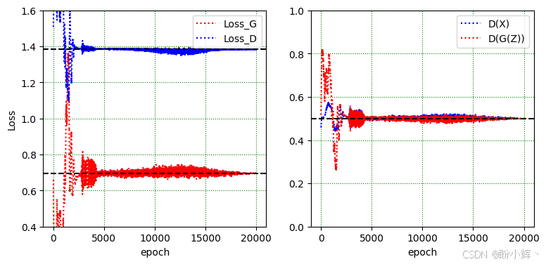

3. 实现生成对抗网络生成 MNIST 图像

本小节将采用上一小节所示的简单双模型 GAN 结构(生成器+判别器)来生成 MNIST 图像。但由于这两个模型的处理能力有限，无法生成与真实 MNIST 图像相媲美的清晰模拟图像。本小节旨在作为对比案例，以此突显下一小节将介绍的深度卷积 GAN 的优越性能。

(1) 首先，导入相关工具库并设置超参数：

import torch
import torch.nn as nn
from torch.utils.data import DataLoader
import torch.optim.lr_scheduler as lr_scheduler
import torchvision.transforms as T
from torchvision.datasets import MNIST
from torchvision.utils import make_grid
import matplotlib.pyplot as plt
import numpy as np
import pandas as pd
from tqdm import trange

n_epochs = 50
batch_size = 100
img_size = 28
img_channels = 1
n_hidden = 128
n_class = 10
z_dim = 100             # Latent space dimensions
lr = 2e-4               # initial learning rate
k = 20                  # k=G_lr/D_lr
fixed_latent = torch.randn(48, z_dim, device='cuda')
path = './data/'

(2) 导入 MNIST 数据集，将数据集切分为批大小为 100 的数据加载器，并在下图中显示第一批图像：

trainData = MNIST(path, train=True, download=False, 
                transform=T.Compose([T.ToTensor(),
                                      T.Normalize([0.5],[0.5])]))                  
n_samples = len(trainData)
train_dataloader = DataLoader(trainData, batch_size=batch_size, shuffle=True)
n_batch = len(train_dataloader)
for imgs, labels in train_dataloader:
    print('batch_imgs.shape=', imgs.shape)
    break
def denorm(img_tensors):          # Shift the value of each image pixel to [0,1]
    return img_tensors * 0.5 + 0.5
def show_imgs(imgs):
    fig, ax = plt.subplots(figsize=(12,8))
    input = make_grid(denorm(imgs[:48]), nrow=16, padding=2) # display 48 images
    ax.imshow(input.permute(1,2,0), cmap='gray')
    ax.set(xticks=[], yticks=[])
    plt.show()
show_imgs(imgs)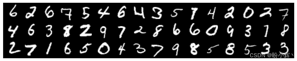

将图像的像素值归一化至 [-1,1] 区间，模型 G 通过 Tanh() 激活函数生成的图像像素值也保持相同范围。执行 imgs.min() 或 imgs.max() 可验证像素值的该取值范围。

尽管 VS Code 在显示这类图像时会提示"将输入数据裁剪至有效范围 [0,1]"，但最好通过 denorm() 函数将像素值转换到 [0,1] 范围。

(3) 定义包含两个全连接层的判别器模型 D 和生成器模型 G，其结构基本与上一小节相同，仅调整了模型 D 的输入变量数和模型 G 的输出变量数：

class Discriminator(nn.Module):
    def __init__(self):
        super().__init__()
        self.model = nn.Sequential(
              nn.Flatten(),           # shape = batch_size x 784
              nn.Linear(img_size*img_size, n_hidden),
              nn.LeakyReLU(0.01),
              nn.Linear(n_hidden, 1),
              nn.Sigmoid())
    def forward(self, images):      
        output = self.model(images)   # images.shape = batch_size x 1 x 28^2
        return output                 # output.shape = batch_size x 1
D = Discriminator().cuda()
class Generator(nn.Module):
    def __init__(self):
        super().__init__()
        self.model = nn.Sequential(
              nn.Linear(z_dim, n_hidden),
              nn.LeakyReLU(0.01),
              nn.Linear(n_hidden, img_size*img_size),
              nn.Tanh())
    def forward(self, z):            # z.shape = batch_size x z_dim
        output = self.model(z)       # output.shape = batch_size x 784
        fake_imgs = output.view(-1, 1, 28, 28)
        return fake_imgs            #fake_imgs = batch_size x 1 x 28^2
G = Generator().cuda()

(4) 当设置 k=1 并采用恒定学习率时，我们发现判别器模型 D 的学习能力优于生成器模型 G。通过引入指数衰减学习率调度器 e − 0.046 i e^{-0.046i} e−0.046i(如下图右侧所示)，并将比例系数 k 设为 20，此时生成器 G 的学习率函数为： G _ l r = k × l r × e − 0.046 i G\_lr = k × lr × e^{-0.046i} G_lr=k×lr×e−0.046i。经过调整，损失函数 Loss_D、G_loss 以及评估指标 D(X) 和 D(G(Z)) 的训练曲线均能收敛至理论值。这种为两个模型分别配置独立学习率调度器的做法是一项重要技巧。

optimizer_D = torch.optim.Adam(D.parameters(), lr=lr, betas=(0.5, 0.999))
optimizer_G = torch.optim.Adam(G.parameters(), lr=k*lr, betas=(0.5, 0.999))
criterion = nn.BCELoss(reduction='sum')
v = lambda i: np.exp(-0.046*i)
scheduler = lr_scheduler.LambdaLR(optimizer_D, lr_lambda=v)
def train_D(inputs, optimizer_D):
    real_preds = D(inputs)
    batch_size = inputs.shape[0]
    one_targets = torch.ones(batch_size, 1, device='cuda')
    real_loss = criterion(real_preds, one_targets)
    real_score = torch.mean(real_preds).item()
    
    z = torch.randn(batch_size, z_dim).cuda()
    fake_images = G(z)
    zero_targets = torch.zeros(batch_size, 1, device='cuda')
    fake_preds = D(fake_images.detach()) 
    fake_loss = criterion(fake_preds, zero_targets)
    fake_score = torch.mean(fake_preds).item()

    loss = real_loss + fake_loss
    optimizer_D.zero_grad()
    loss.backward()
    optimizer_D.step()
    return loss.item(), real_score, fake_score
def train_G(optimizer_G):
    z = torch.randn(batch_size, z_dim).cuda()
    fake_images = G(z)    # Create fake images
    preds = D(fake_images)      
    one_targets = torch.ones(batch_size, 1).cuda()
    # Try to fool the discriminator
    loss = criterion(preds, one_targets)
    optimizer_G.zero_grad()
    loss.backward()
    optimizer_G.step()
    return loss.item()
def fit(epochs):
    torch.cuda.empty_cache()
    df = pd.DataFrame(np.empty([epochs, 5]), 
        index = np.arange(epochs),
        columns=['Loss_G', 'Loss_D', 'D(X)', 'D(G(Z))', 'LearningRate']) 
    for i in trange(epochs):
        loss_G = 0.0; loss_D = 0.0; real_sc = 0.0; fake_sc = 0.0
        for real_images, _ in train_dataloader:    
            inputs = real_images.cuda()
            loss_d, real_score, fake_score = train_D(inputs, optimizer_D)
            loss_D += loss_d; real_sc += real_score; fake_sc += fake_score
            loss_g = train_G(optimizer_G)
            loss_G += loss_g
        df.iloc[i, 0] = loss_G/n_samples
        df.iloc[i, 1:4] = loss_D/n_samples, real_sc/n_batch, fake_sc/n_batch
        df.iloc[i, 4] = optimizer_D.param_groups[0]['lr']       #Record lr_D
        scheduler.step()                                        #Update lr_D
        optimizer_G.param_groups[0]['lr'] = df.iloc[i,4]*k #------------line 18
        if i==0 or (i+1)%5==0:
            print(
            "Epoch={}, Ls_G={:.4f}, Ls_D={:.4f}, D(X)={:.4f}, D(G(Z))={:.4f}"
            .format(i+1, df.iloc[i,0], df.iloc[i,1], df.iloc[i,2], df.iloc[i,3]))
            fake_images = G(fixed_latent)
            show_imgs(fake_images.detach().cpu())        
    return df
train_history = fit(n_epochs)    #dt = 10 min, n_epochs=50
df= train_history
fig, ax = plt.subplots(1,3, figsize=(15,4), sharex=True)
df.plot(ax=ax[0], y=[0,1], style=['r-+', 'b-'])
df.plot(ax=ax[1], y=[2,3], style=['b-', 'r-+'])
df.plot(ax=ax[2], y=[4], style=['r-+'])
for i in range(3):
    ax[i].set_xlabel('epoch')
    ax[i].grid(which='major', axis='both', color='g', linestyle=':')
ax[0].set(ylabel='Loss', ylim=[0.4,1.8])
ax[0].axhline(y=2*np.log(2), color='k', linestyle='--') #Theory D loss Value
ax[0].axhline(y=np.log(2), color='k', linestyle='--')   #Theory G loss Value
ax[1].axhline(y=0.5, color='k', linestyle='--')         #Theory D(X), D(G(Z)) values
ax[1].set_ylim([0.48, 0.6])
ax[2].set_ylim([0, 2.2e-4])
ax[2].ticklabel_format(style='sci', axis='y', scilimits=(0,0));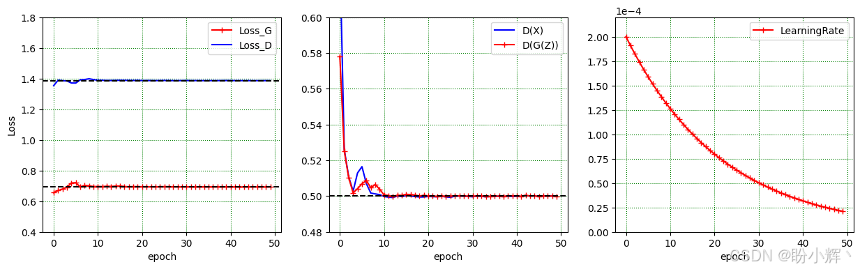

小结

本节介绍了生成对抗网络 (Generative Adversarial Network, GAN) 的理论基础与实现方法。GAN 通过生成器与判别器的对抗博弈，使生成器逐步学习真实数据分布，最终生成以假乱真的样本。理论部分详细推导了最优判别器表达式及损失函数界限。实践环节首先在二次曲线数据集上验证了 GAN 训练框架，损失曲线与理论值高度吻合。随后将简单全连接 GAN 应用于 MNIST 手写数字生成，通过为生成器设置更高学习率 (k=20) 并采用指数衰减调度器，有效平衡了双模型训练，使 D(X) 和 D(G(Z)) 收敛至理论值 0.5。

系列链接

PyTorch计算机视觉（1）------计算机视觉的数学工具

PyTorch计算机视觉（2）------神经网络模型训练与PyTorch基础

PyTorch计算机视觉（3）------卷积神经网络（CNN）详解与实现

PyTorch计算机视觉（4）------迁移学习（Transfer Learning）详解与实现