Pytorch图模式技术原理解析

作者 ：昇腾实战派

知识地图：https://blog.csdn.net/Lumos_Lovegood/article/details/161601003

背景概述

在深度学习框架中，图模式通过将模型计算编译为高效内核来提升执行性能，是 PyTorch 2.x 的核心能力。本文系统解析了 PyTorch 图模式的整体技术原理，涵盖 TorchDynamo 字节码捕获、AOTAutograd 前反向图生成、TorchInductor 算子融合与内核生成等关键环节，并以端到端示例展示编译加速效果，为理解图模式编译流程与进行性能优化提供参考。

Eager模式

在PyTorch中，"eager模式"是指PyTorch的默认执行模式，其中每个操作都是即时执行的，与Python的执行流程紧密集成。这与早期的深度学习框架（如TensorFlow 1.x）使用的静态计算图模式形成对比，后者需要先定义一个计算图，然后在整个图被完全定义后才能执行。

eager模式允许开发者以更直观和交互式的方式进行深度学习模型的开发和调试。以下是一些关于PyTorch eager模式的关键点：

1. 即时执行：在eager模式下，操作（如加减乘除、矩阵乘法等）会立即执行并返回结果，这与Python的标准执行方式一致。
2. 直观的错误调试：由于操作是即时执行的，因此如果代码中有错误，PyTorch会立即抛出异常，这使得错误调试更加直接和简单。
3. 动态计算图：在eager模式下，计算图是动态构建的，这意味着图的形状和大小可以在运行时改变，这为处理复杂的模型结构和控制流提供了极大的灵活性。
4. 自动微分（Autograd）：PyTorch的eager模式与自动微分机制（Autograd）紧密结合，可以自动计算梯度，这对于实现神经网络的反向传播至关重要。
5. 易于使用：eager模式下的PyTorch代码更容易阅读和理解，因为它更接近于标准的Python编程方式。
6. 与Python深度集成：eager模式允许开发者使用Python的调试工具和库，如pdb，以及利用Python的交互式特性，如Jupyter notebooks，来探索和实验。

总的来说，PyTorch的eager模式为深度学习研究者和开发者提供了一种更加灵活、直观和高效的开发体验。这种模式使得PyTorch成为深度学习领域最受欢迎的框架之一。

图模式

PyTorch图模式与PyTorch的默认eager模式形成对比，在eager模式中，每个操作都是即时执行的。

图模式在某些情况下可以提高性能和效率，尤其是当模型的结构固定，且需要重复执行多次时。

PyTorch更新到2.x之后引入了一系列与AI编译器相关的组件，全面开启图模式生态。

通过torch.compile(model.forward)这一行代码可以开启图模式，将PyTorch function进行编译加速。

torch.compile整体流程

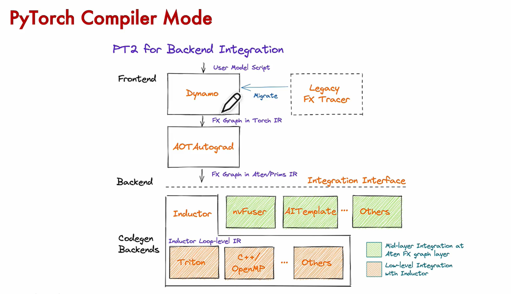
Dynamo：前端 ------ 从 Python 代码 到 FX Graph（前向）

AOTAutograd：中端 ------ 从前向图生成反向图，并做图变换

Inductor: 后端 ------ 将图编译成高效内核。

torch.compile(model)

│

├─ 1 TorchDynamo 字节码拦截 → FX Graph 捕获 → Guard 生成

│

├─ 2 AOTAutograd 函数化 → 算子分解 → 联合图 → 最小割分区

│

├─ 3 TorchInductor FX → Inductor IR → Fusion Scheduler → Memory Planning

│

├─ 4 Triton Codegen IR → @triton.jit kernel → Autotuning → PTX → cubin

│

└─ 5 Runtime Guard check → cache lookup → kernel launch

TorchDynamo

import torch
from typing import List

def my_compiler(gm: torch.fx.GraphModule, example_inputs: List[torch.Tensor]):
    print(">>> FX graph:")
    gm.graph.print_tabular()
    print(f">>> Code:\n{gm.code}")
    return gm.forward  # return a python callable

@torch.compile(backend=my_compiler)
def f(x: torch.Tensor):
    b = torch.floor(x) + torch.ceil(x)
    c = b.sum(dim=-1)
    d = c + 1
    return d

if __name__ == "__main__":
    ret = f(torch.ones([32,512,1024], device="cuda"))

执行上面的代码，可以看到 TorchDynamo 把从函数 foo() 中捕获到一张计算图，TorchDynamo 以 FX Graph 保存捕获到的计算图:

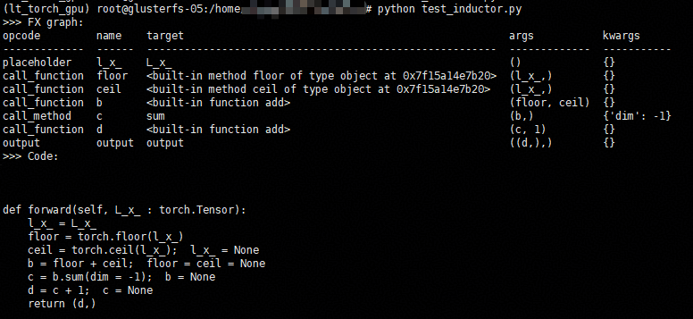
Torch Dynamo会解释运行f的Python Bytecode，捕捉到对应FX Graph

Python 字节码

TorchDynamo 捕获计算图是在翻译 Python 字节码的过程中实现的。Python 函数在执行前会被 Python 虚拟机编译为字节码 (bytecode)，每一个 Python 函数的实例都对应一个 frame，其中保存着运行该函数所需要的全局变量、局部变量、字节码等等。

为了便于理解 Python 虚拟机、字节码和 TorchDynamo 的行为，下面用 hello() 函数简要介绍下 Python 字节码的行为。可以用 dis 包查看 Python 函数的字节码:

import dis

def hello():
    print("Hello, world!")

for k in ["co_names", "co_varnames", "co_consts"]:
    print(k, getattr(hello.__code__, k))
print(dis.dis(hello))

执行上面的代码，我们得到下面的结果:

co_names ('print',)
co_varnames ()
co_consts (None, 'Hello, world!')

0 LOAD_GLOBAL              0 (print)
2 LOAD_CONST               1 ('Hello, world!')
4 CALL_FUNCTION            1
6 POP_TOP
8 LOAD_CONST               0 (None)
10 RETURN_VALUE

其中包含了 6 条 Python 字节码，它们的功能如下:

• LOAD_GLOBAL 0: 从 f_builtins 和 f_globals 中加载由下标 0 所引用的全局对象，把它压到数据栈上;
• LOAD_CONST 1: 从 co_consts 中加载由下标 1 所引用的常量，把它压到数据栈上;
• CALL_FUNCTION 1: 从栈顶出栈 1 个元素作为函数参数，再出栈一个元素作为被调函数，调用该函数并把返回值压到数据栈上；
• POP_TOP: 从栈顶移除一个元素;
• LOAD_CONST 0: 从 co_consts 中加载由下标 0 所引用的常量，把它压到数据栈上;
• RETURN_VALUE: 从栈顶出栈 1 个元素，把它作为返回值返回给主调函数;

Python 虚拟机是 Stack Machine，它维护了 3 个 stack：

• Call Stack: 其中的条目是 Python frame，类似 C 的函数调用栈；
• Evaluation Stack (or Data Stack): 每个 Python frame 都有一个 evaluation stack，执行 Python 字节码时的数据由该 stack 管理，这与常见的 Register Machine 有所区别；
• Block Stack : 每个 Python frame 都有一个 block stack，目的是跟踪 Python 中的控制结构，例如循环、try / except、with 语句等，进入/退出这类控制结构时会有对应的条目被 push/pop。Block stack 帮助 Python 在任意时刻都知道当前活跃的 block，continue 和 break 会影响当前活跃的 block；

实现原理

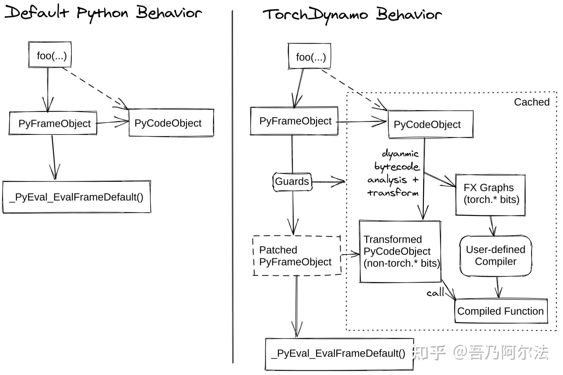
TorchDynamo 的 编译过程发生在将要执行前 ，它是一个 JIT 编译器。在 Python 将要执行函数时，TorchDynamo 开始翻译字节码并捕获计算图。在 Python 虚拟机 (PVM) 中有一个非常重要的函数 _PyEval_EvalFrameDefault，它的功能是在 PVM 中逐条执行编译好的字节码。TorchDynamo 的入口是 PEP-523 提供的 CPython Frame Evaluation API，它可以让用户通过 回调函数（callback function） 获取字节码，并把修改过后的字节码返回给解释器执行，或者执行预先编译好的目标代码，从而可以在 Python 中实现 即时编译器 (JIT Compiler) 的功能。TorchDynamo 正是通过 PEP-523 把 TorchDynamo 的核心逻辑引入到 Python 虚拟机中，从而在函数将要运行前获取字节码。

TorchDynamo 实现了一个 Python 虚拟机的模拟器，在模拟 Python 字节码执行的过程中构建出对应的计算图 。仍以 foo() 为例:

@torch.compile(backend=my_compiler)
def foo(x, y):
    return (x + y) * x

foo() 对应的字节码如下，TorchDynamo 在翻译字节码 BINARY_ADD 和 BINARY_MULTIPLY 时在 FX Graph 中建立了 operator.add 和 operator.mul 两个 FX Node，最后形成一张完整的计算图:

0 LOAD_FAST                0 (x)
 2 LOAD_FAST                1 (y)
 4 BINARY_ADD
 6 LOAD_FAST                0 (x)
 8 BINARY_MULTIPLY
10 RETURN_VALUE

为了检验 TorchDynamo 捕获的计算图在下次执行时还是否有效，TorchDynamo 会为被编译的函数创建 Guard。从 Guard 生成的 Python 可执行函数 check_fn，在 TorchDynamo 中 负责检测被编译函数的输入属性是否发生变化 ，如果没有发生变化则可以重用此前编译好的函数，否则当前输入对此前编译好的函数无效，需要 重新编译 (graph recompilation) 该函数。TENSOR_MATCH 是检测张量信息的 Guard，在默认情况下，主要负责检查输入的张量 device、shape、stride 等属性是否改变。

foo() 函数对应的 check_fn 如下，它会调用 C++ 函数检查张量 x 和 y 的信息是否发生变化，进而决定是否能重用此前编译好的函数:

GUARDS ___guarded_code.valid and ___check_tensors(x, y)

经 TorchDynamo 编译好的函数被保存在 frame 的 cache 中，从而避免再次编译相同的函数和输入。默认情况下 cache 大小为 64，也就是说，对于同一个 Python 函数，它的输入最多可以有 64 种变化，超过这个限制后 Dynamo 就不再编译，直接降级回 Eager 模式，避免缓存爆炸。

动态shape

默认情况下 TorchDynamo 为 static shape 模式，捕获计算图时张量的 shape 和 stride 被特化并记录在 Guard 中。捕获计算图结束时会生成 Guard 对应的 check_fn，用于 检查该计算图中的输入信息有没有发生变化 。如果没有发生变化则重用已经编译好的计算图，否则重新捕获并编译计算图 (graph recompilation)。当设置环境变量 TORCHDYNAMO_DYNAMIC_SHAPES 为 1 时，此时 TorchDynamo 以 dynamic shape 模式捕获计算图，张量的 shape 和 stride 不会被特化、不会被记录在 Guard 中，生成的 check_fn 也不检查 shape 和 stride。因此，以不同 shape 或 stride 的张量执行编译好的计算图时，不会重新捕获计算图和重新编译。

下面的代码片段中，test() 调用了两次 toy_example()，两次不同的调用之间 tensor 的 shape 不同，所以会触发重新编译:

@torch.compile(backend=my_compiler)
def toy_example(x):
    x = x / (torch.abs(x) + 1)
    return x

def test():
    x = torch.randn(10)
    toy_example(x)
    x = torch.randn(20)
    toy_example(x)

AOTAutograd

AOTAutograd会根据这张forward FX Graph，生成计算backward pass的FX Graph。在这个过程中，可能会有Pattern Matcher优化掉图中的一部分。一些比较复杂的Op，会通过decomposition拆成更简单的Op

在 PyTorch 2.0 以前，用户通过 PyTorch 可以直接捕获到正向传播的计算图，比如 JIT trace 和 TorchFX 的 symbolic trace。虽然 PyTorch 的每个算子都包含正向传播和反向传播的实现，但用户并不能直接在反向传播的计算图上面做优化，也无法把正向传播和反向传播的计算图合并在一张计算图中。PyTorch 2.0 中引入了 AOTAutograd，它的出现解决了这个问题，从而使得一些针对 training 的优化变得可能。

有了 AOTAutograd，用户可以做以下事情:

• 获取反向传播计算图、甚至是正向传播和反向传播联合的计算图;
• 用不同的后端编译器分别编译正向传播和反向传播计算图;
• 针对训练 (training) 做正向传播、反向传播联合优化，比如通过在反向传播中重算 (recompute) 来减少正向传播为反向传播保留的 tensor，从而削减内存需求;

总的来说，AOTAutograd的工作流程如下：

1. 基于torch_dispatch机制trace正向反向传播，生成联合计算图（joint graph）。
2. 通过decompositions进一步拆解，将FX Graph进一步转换为更低层次的中间表示，即PrimTorch。
3. 通过partition_fn将joint-graph切分成正反向计算图。
4. 调用fw_compiler和bw_compiler对正向、反向计算图分别进行编译，并整合成一个torch.autograd.Function。

import torch
from functorch.compile import aot_function, \
    make_boxed_func, ts_compile

def fn(a, b, c, d):
    x = a + b + c + d
    return x.cos().cos()

def run_func(func, *inputs):
    res = func(*inputs)
    loss = res.sum()
    loss.backward()

def compiler_fn(fx_module: torch.fx.GraphModule, _):
    print(fx_module.code)
    return make_boxed_func(fx_module.forward)

a, b, c, d = [torch.randn(2, 4, requires_grad=True,
    device="cuda") for _ in range(4)]
run_func(fn, a, b, c, d)

aot_print_fn = aot_function(fn, fw_compiler=compiler_fn,
    bw_compiler=compiler_fn)
run_func(aot_print_fn, a, b, c, d)

AOTAutograd自动切分前反向联合计算图图，得到前向图和反向图，AOTAutograd默认使用了 min_cut_rematerialization_partition，它的作用是针对前向传播计算图和反向传播计算图做联合优化，从而降低内存需求**😗*

def forward(self, primals_1, primals_2, primals_3, primals_4):   # 前向图
    add = torch.ops.aten.add.Tensor(primals_1, primals_2);  primals_1 = primals_2 = None
    add_1 = torch.ops.aten.add.Tensor(add, primals_3);  add = primals_3 = None
    add_2 = torch.ops.aten.add.Tensor(add_1, primals_4);  add_1 = primals_4 = None
    cos = torch.ops.aten.cos.default(add_2)
    cos_1 = torch.ops.aten.cos.default(cos)
    return [cos_1, cos, add_2]

def forward(self, cos, add_2, tangents_1):  # 反向图
    sin = torch.ops.aten.sin.default(cos);  cos = None
    neg = torch.ops.aten.neg.default(sin);  sin = None
    mul = torch.ops.aten.mul.Tensor(tangents_1, neg);  tangents_1 = neg = None
    sin_1 = torch.ops.aten.sin.default(add_2);  add_2 = None
    neg_1 = torch.ops.aten.neg.default(sin_1);  sin_1 = None
    mul_1 = torch.ops.aten.mul.Tensor(mul, neg_1);  mul = neg_1 = None
    return [mul_1, mul_1, mul_1, mul_1]

自定义的编译器 compiler_fn() 被调用了两次，分别打印正向传播和反向传播计算图对应的 Python 代码。其中的 primals 和 tangents 是微分几何中的概念，可以把 primals 理解为用户函数的输入，它是正向传播的输入，把 tangents 理解为用户函数输出的梯度，它是反向传播的输入。两张计算图是 FX Graph，其中包含的是 ATen 算子，它们是 low-level 算子，而不是 Torch 级别的算子，例如 Linear。

PyTorch 反向传播的计算图是在执行正向传播的过程中动态构建的，反向传播的计算图在正向传播结束时才能确定下来。AOTAutograd 以 Ahead-of-Time 的方式同时 trace 正向传播和反向传播，从而在函数真正执行之前拿到正向传播和反向传播的计算图。

AOTAutograd 的工作流程 如下:

• 以 AOT 方式通过 __torch_dispatch__ 机制 trace 正向传播和反向传播，生成联合计算图 (joint forward and backward graph)，它是包含 Aten/Prim 算子的 FX Graph;
• 用 partition_fn 把 joint graph 划分为正向传播计算图和反向传播计算图;
• 可选: 通过 decompositions 把 high-level 算子分解、下沉到粒度更小的算子;
• 调用 fw_compiler 和 bw_compiler 分别编译正向传播计算图和反向传播计算图，通过 TorchFX 生成编译后的 Python 代码，并整合为一个 torch.autograd.Function;

torch_dispatch

AOTAutograd是基于torch_dispatch机制在算子下发执行前获得真正实际执行的op，并构建对应的Proxy，即PyTorch反向传播的计算图是在执行正向过程中动态创建的，这也意味着执行完整的前向过程才能构建出对应的FX Graph，从而在函数正式执行前拿到正反向计算图，实现AOTAutograd，而这一过程也是依赖于前面TorchDynamo捕获的FX Graph这一IR表示。

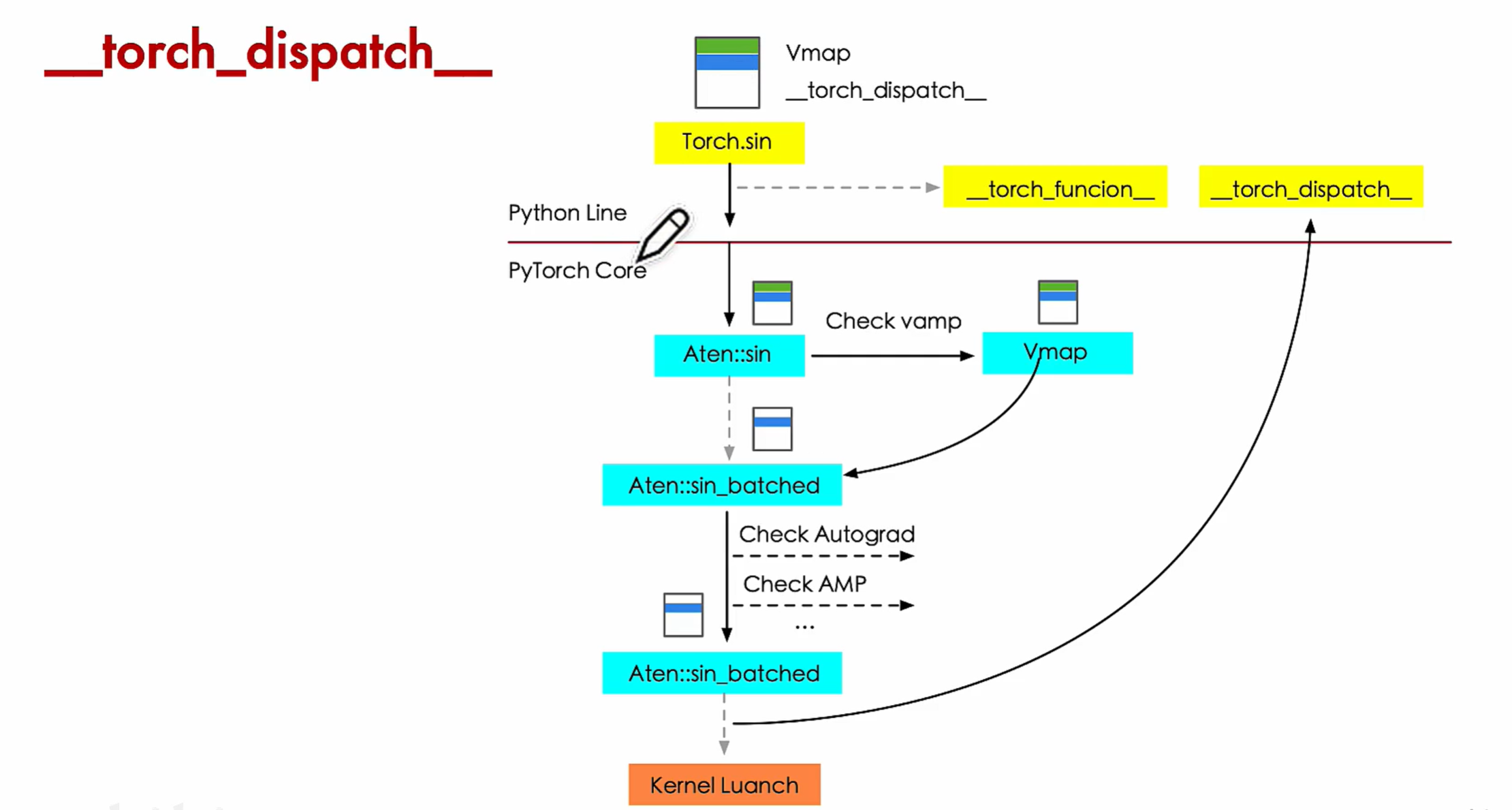
红线分开python和Pytorch核心，python代码不是马上执行，执行sin函数操作会先走到aten算子然后进行一层封装，然后进行Autograd，AMP的操作，最后在kenerl Luanch之前去调用__torch_dispatch__，可以看到整个操作都是在python层面完成的。(一些比较复杂的Op，会通过decomposition拆成更简单的Op)

# __torch_dispatch__执行过程
    r = maybe_handle_decomp(proxy_mode, func, args, kwargs)    # 基于CURRENT_DECOMPOSITION_TABLE查找op对应的函数实现并返回
    if r is not NotImplemented:
        return r

    # 不是ATen op则进一步拆解算子
    # For pre-autograd tracing, we do not want to run CompositeImplicit decomps.
    if not pre_dispatch and func not in [
        torch.ops.aten.size.default,
        torch.ops.aten.stride.default,
        torch.ops.aten.storage_offset.default,
    ]:
        with proxy_mode:
            r = func.decompose(*args, **kwargs)
            if r is not NotImplemented:
                return r
    # 对中间函数调用创建类型为call_function的Proxy
    proxy_args, proxy_kwargs = pytree.tree_unflatten(proxy_flat_args_kwargs, spec)
    proxy_out = proxy_mode.tracer.create_proxy(
        "call_function",
        func,
        proxy_args,
        proxy_kwargs,
        name=proxy_mode.tracer.graph._target_to_str(func.overloadpacket.__name__),
    )

    out = func(*args, **kwargs)    # 以FakeTensor作为输入运行函数拿到对应的输出
    track_tensor_tree(out, proxy_out, constant=constant, tracer=tracer)    # 将结果Tensor绑定到对应Proxy中
    return out

def track_tensor_tree(inner_res, proxy_res, *, constant, tracer):
    def wrap_with_proxy(e, proxy, constant):
        if isinstance(e, torch.Tensor):
            track_tensor(e, proxy, tracer=tracer, constant=constant)
            set_meta(proxy, e)
        elif isinstance(e, py_sym_types):
            # NB: eagerly set meta here, so that the numbering is in order
            set_meta(proxy, e)
            set_proxy_slot(e.node, tracer, lambda: proxy)
        elif isinstance(e, list):
            # example use case: allreduce_ returns ([tensor], work)
            for idx, ee in enumerate(e):
                wrap_with_proxy(ee, proxy[idx], get_constant(idx))

def create_proxy(self, kind: str, target: Target, args: Tuple[Any, ...], kwargs: Dict[str, Any],
       ame: Optional[str] = None, type_expr : Optional[Any] = None,
       proxy_factory_fn: Callable[[Node], 'Proxy'] = None):

       args_ = self.create_arg(args)
       kwargs_ = self.create_arg(kwargs)

       node = self.create_node(kind, target, args_, kwargs_, name, type_expr) 

       if not proxy_factory_fn:
           proxy = self.proxy(node)
       else:
           proxy = proxy_factory_fn(node) 
 
       return proxy

Proxy 是一个代理对象（Proxy Object），它的核心作用是：在不执行真实计算的情况下，拦截并记录对张量（或其它对象）的所有操作，从而构建一个计算图

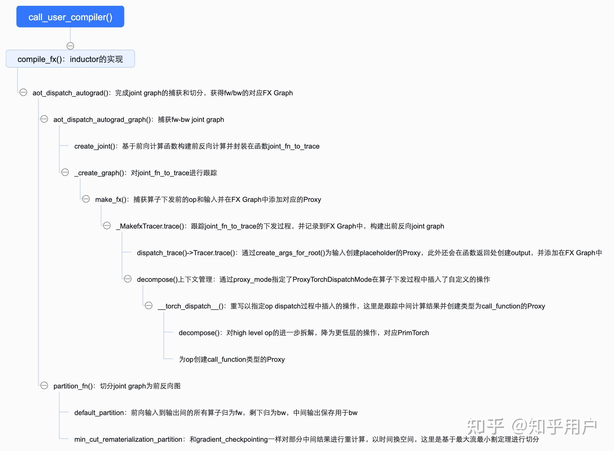
通过上面的torch_dispatch和_MakefxTracer.trace()跟踪，从而在整个joint_fn_to_trace执行完毕后将所有操作都记录到FX Graph中，构建出正反向joint graph。并在_MakefxTracer.trace()中通过fx._lazy_graph_module._make_graph_module(tracer.root, graph, name)生成GraphModule并一路返回到aot_dispatch_autograd_graph()，对joint graph通过eliminate_dead_code()进行冗余代码消除和recompile()生成对应python代码，并返回到aot_dispatch_autograd()进行后续的切分。

autograd调用函数

Joint Graph

aot_dispatch_autograd_graph()函数生成joint graph的过程：

1. 通过create_joint()函数将正反向计算封装成函数，create_joint()根据前向计算结果分析出需要计算梯度的参数以及对应的tangents（梯度权值），然后通过torch.autograd.grad进行反向求导，并将正反向过程封装在函数中返回，作为joint_fn_to_trace。
2. 由_create_graph()对joint_fn_to_trace函数进行跟踪，核心是调用make_fx()函数在算子dispatch前拿到实际真正执行的op并创建Proxy添加到FX Graph中。

在make_fx()函数中是通过_MakefxTracer.trace()函数对整个函数计算过程进行跟踪并生成GraphModule，GraphModule中包含正反向计算对应的计算图。需要注意的是这里的正反向计算是TorchDynamo graph break对应的子图，即每个子图都会调用一次make_fx生成joint graph。捕获过程主要包括两个核心操作： 1）对输入输出的封装：在dispatch_trace()->Tracer.trace()中会为函数参数、局部变量以及输出生成对应的Proxy。其中通过create_args_for_root()->create_proxy()为所有变量（函数参数和局部变量）创建类型为placeholder的Proxy，在create_proxy()中会同步创建Node并将其加入到FX Graph中，并用Proxy封装一下Node。通过create_node()为输出创建类型为 output 的Node，并将其加入到FX Graph中）。 2）op dispatch的捕获和封装： 在with decompose()上下文管理中通过self.proxy_mode指定了ProxyTorchDispatchMode（用于拦截和自定义张量操作的分发过程，Dispatch Mode 机制允许开发者在张量操作（如加法、矩阵乘法等）被执行时，插入自定义逻辑，以实现诸如调试、性能监控、自定义后端支持等功能，而不需要修改Python的核心代码）。通过重写torch_dispatch函数指定op dispatch过程中插入的操作，在ProxyTorchDispatchMode中是对op的decompose（拆解到PrimTorch规定的集合中），同时为op创建类型为call_function()的Proxy。

make_fx

AOTAutograd 通过 make_fx 来 trace 该 joint_forward_backward 函数，对于其中的每个算子，都会触发 torch_dispatch，从 tensor 获取 proxy，在 fx.Graph 中创建算子对应的 proxy，类型为 call_function，目标是算子本身，然后以真实 tensor 运行算子，并把结果 tensor 绑定到 proxy 上:如此往复，直到 AOTAutograd trace 完正向传播和反向传播中的所有算子，得到一张完整的 joint graph

flattened_joints, _ = pytree.tree_flatten(joint_inputs) fx_g = make_fx(joint_forward_backward, aot_config.decompositions)( *joint_inputs )

flattened_joints, _ = pytree.tree_flatten(joint_inputs)
            fx_g = make_fx(joint_forward_backward, aot_config.decompositions)(
                *joint_inputs
            )

assert tracing_mode in ["real", "fake", "symbolic"]
    if decomposition_table is None:
        decomposition_table = {}

        proxy_mode = ProxyTorchDispatchMode(fx_tracer, tracing_mode)

        arg_count = 0
        def wrap_fake(x):
            nonlocal arg_count
            if isinstance(x, torch.Tensor):
                from torch._dynamo.source import ConstantSource
                source = ConstantSource(f"input{arg_count}")
                arg_count += 1
                return fake_tensor_mode.from_tensor(x, source=source)  # type: ignore[attr-defined]
            return x

        sym_mode = proxy_mode.sym_mode

        wrap_fn_map = {
            "real": lambda x: x,
            "fake": wrap_fake,
            "symbolic": wrap_fake,
        }
        args = pytree.tree_map(wrap_fn_map[tracing_mode], args)

        with decompose(decomposition_table), fake_tensor_mode, python_dispatcher_mode, \
             sym_mode, proxy_mode, disable_autocast_cache(), disable_proxy_modes_tracing(enable_current=True):
            t = dispatch_trace(wrap_key(func, args, fx_tracer), tracer=fx_tracer, concrete_args=tuple(phs))
        return t

    return wrapped

dispatch_trace

def dispatch_trace(
        root: Union[torch.nn.Module, Callable],
        tracer: Tracer,
        concrete_args: Optional[Tuple[Any, ...]] = None,
) -> GraphModule:
    graph = tracer.trace(root, concrete_args)
    name = root.__class__.__name__ if isinstance(root, torch.nn.Module) else root.__name__
    return GraphModule(tracer.root, graph, name)

Tracer 类

Tracer 类的核心作用是：对一个函数或 torch.nn.Module 的执行过程进行追踪（tracing），并将其转换为一个中间表示（Intermediate Representation, IR）------即 Graph 对象。这个 Graph 可用于后续的分析、变换、优化或代码生成。

Tracer.trace()

PyTorch FX（torch.fx）中 symbolic tracing 的核心实现，用于将一个 nn.Module 或普通函数转换为可分析、可修改、可执行的计算图（torch.fx.Graph）

self.create_node( "output", "output", (self.create_arg(fn(*args)),), {}, type_expr=fn.__annotations__.get("return", None), )

torch_dispatch（即 torch_dispatch）是在执行 Proxy 对象上的 PyTorch 操作时，由 PyTorch 的 调度器（Dispatcher） 自动调用的。

partition

# joint-graph示例
============original joint graph
opcode         name        target            args               kwargs
-------------  ----------  ----------------  -----------------  --------
placeholder    primals_1   primals_1         ()                 {}
placeholder    tangents_1  tangents_1        ()                 {}
call_function  cos         aten.cos.default  (primals_1,)       {}
call_function  cos_1       aten.cos.default  (cos,)             {}
call_function  sin         aten.sin.default  (cos,)             {}
call_function  neg         aten.neg.default  (sin,)             {}
call_function  mul         aten.mul.Tensor   (tangents_1, neg)  {}
call_function  sin_1       aten.sin.default  (primals_1,)       {}
call_function  neg_1       aten.neg.default  (sin_1,)           {}
call_function  mul_1       aten.mul.Tensor   (mul, neg_1)       {}
output         output      output            ([cos_1, mul_1],)  {}
======================forward graph
opcode         name       target            args                   kwargs
-------------  ---------  ----------------  ---------------------  --------
placeholder    primals_1  primals_1         ()                     {}
call_function  cos        aten.cos.default  (primals_1,)           {}
call_function  cos_1      aten.cos.default  (cos,)                 {}
output         output     output            ([cos_1, primals_1],)  {}
======================backward graph
opcode         name        target            args               kwargs
-------------  ----------  ----------------  -----------------  --------
placeholder    primals_1   primals_1         ()                 {}
placeholder    tangents_1  tangents_1        ()                 {}
call_function  cos         aten.cos.default  (primals_1,)       {}
call_function  sin         aten.sin.default  (cos,)             {}
call_function  neg         aten.neg.default  (sin,)             {}
call_function  mul         aten.mul.Tensor   (tangents_1, neg)  {}
call_function  sin_1       aten.sin.default  (primals_1,)       {}
call_function  neg_1       aten.neg.default  (sin_1,)           {}
call_function  mul_1       aten.mul.Tensor   (mul, neg_1)       {}
output         output      output            ([mul_1],)         {}
======================end

Torch Inductor

TorchInductor 是 PyTorch 的一个高性能编译后端，专注于将优化后的计算图转换为高效的、针对特定硬件（如 CPU、GPU）的内核代码。它利用多种优化技术，包括内存优化、并行化和低层次的代码生成，以最大化计算性能。aot_dispatch_autograd()函数在拿到前反向的FX Graph后，分别调用fw_compiler、bw_compiler对前反向图进行编译，这里的fw_compiler和bw_compiler可以是不同的compiler，在inductor的默认实现中调用的是compile_fx_inner，而其中的核心函数是fx_codegen_and_compile()，负责对FX Graph进行图优化、Triton内核代码生成等。

post_grad_passes

https://github.com/pytorch/pytorch/blob/main/torch/_inductor/fx_passes/post_grad.py

以递归的方式处理每个子图，处理逻辑如下：

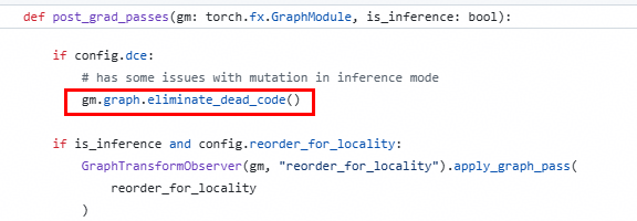
1. 消除死代码 ，eliminate_dead_code
   遍历整个graph的节点，如果不是输出节点，且没有节点依赖于当前节点输出，则这个节点可以去掉。
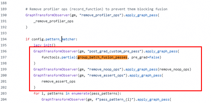
2. **识别和融合可以批量处理的操作。**初始时post_grad_fusion_options为空，在运行时会注册batch_aten的加减乘除pattern；接着generate_fusion_from_config查看是否有相应的配置信息，然后遍历所有规则，进行匹配，匹配到了就进行更新graph的node；有了配置信息，再从注册的表里面拿到对应的规则对象
3. 消除无意义的算子 remove_noop_ops，从node表中读取placeholder 节点，遍历所有node，将满足表达式的node，在保证不破坏输入与输出见内存共享关系和试图中的现有别名的条件下进行替换；首先若能有效提取node中的参数时且发现当前节点与源节点的元数据相同且替换前后不改变程序语义，则所有对当前节点的引用替换为对源节点的引用并删除当前节点
4. 删除断言 remove_assert_ops ，断言不影响计算，但会阻止融合
5. 执行 3 轮算子融合 （pass_patterns 0/1/2）
   运行
   for i, patterns in enumerate(pass_patterns):
   patterns.apply(graph)
   包含：
   softmax 在线优化
   mm + mm 融合
   add + mm → addmm
   split + cat 消除
   各种逐点算子融合
6. 分解高阶算子：decompose_auto_functionalized：对high-level op进一步进行拆解（因为前面进行算子融合那些操作可能会引入新的high level op所以这里再操作一遍），将高层次的操作逐步转换为更低层次的实现。

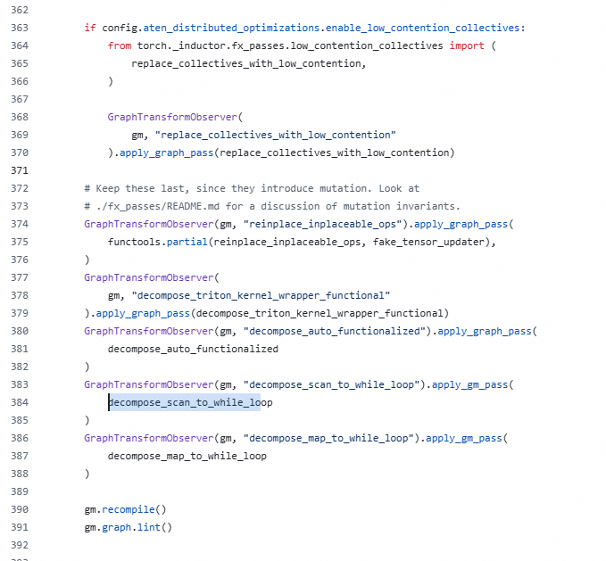
最后重新编译更新fx图

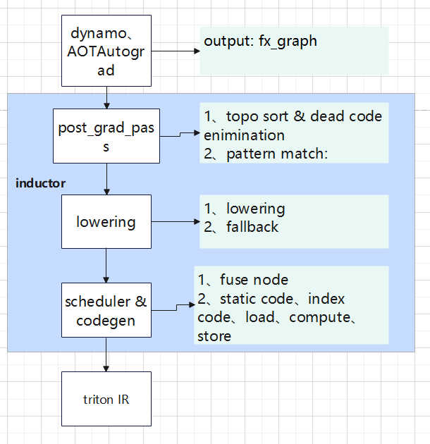
post_grad_passes 的核心任务：把 FX 图里的小 ATen 算子尽量合并、清理、重排，为后续 Lowering 成 Pointwise/Reduction/Fusion IR 做准备。

lowering

https://github.com/pytorch/pytorch/blob/main/torch/_inductor/compile_fx.py

主要功能：把FX Graph进一步降为Inductor IR，即前面的计算图被进一步转换为低层次的中间表示(将输入翻译成pointwise/computeBuffer的Loop level IR)。这一表示更加接近最终的机器代码，并且适合进一步的代码生成和优化。

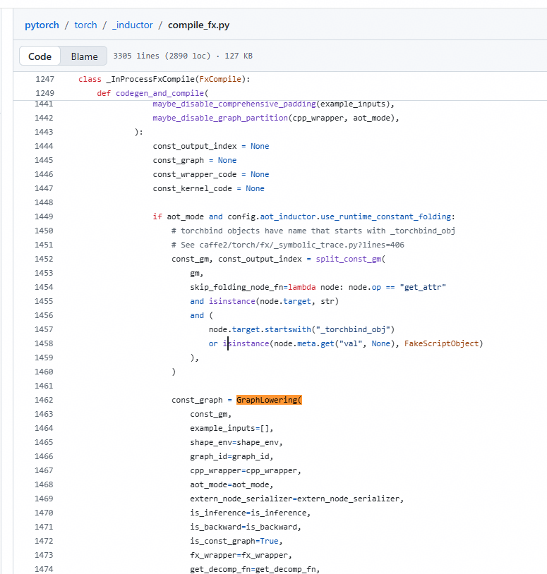
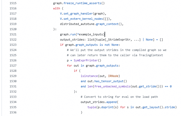
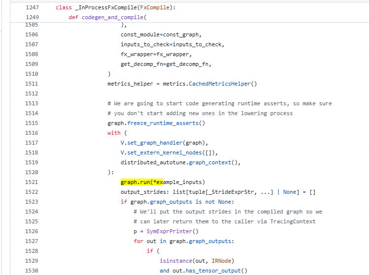
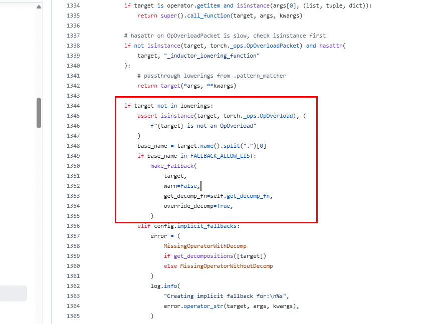
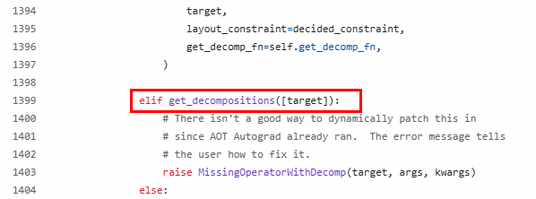
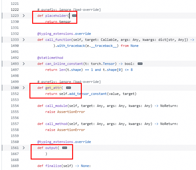
在graph.run(*example_inputs)中对graph的每一个node进行转换生成每一步的inductor ir，主要实现通过每一个node中op然后调用lower中对应的函数实现初步inductor ir的生成。（如果不在lowering中，检测是否存在于白名单和implicit_fallbacks配置），最后根据node.op找到执行的函数，然后就被解释器调用到class GraphLowering(torch.fx.Interpreter):的下面的函数里

Inductor IR到Triton的转化

Pointwise测试用例

@torch.compile
def fa(x: torch.Tensor):
    a = torch.floor(x) + torch.ceil(x)
    return a
fa(torch.empty([32,512,1024], device="cuda"))

打印出IR信息

ComputedBuffer(
    name='buf0', 
    layout=FixedLayout('cuda', torch.float32, size=[32, 512, 1024], stride=[524288, 1024, 1]), 
    data=Pointwise(
        'cuda',
        torch.float32,
        def inner_fn(index):
            i0, i1, i2 = index
            tmp0 = ops.load(arg0_1, i2 + 1024 * i1 + 524288 * i0)
            tmp1 = ops.floor(tmp0)
            tmp2 = ops.load(arg0_1, i2 + 1024 * i1 + 524288 * i0)
            tmp3 = ops.ceil(tmp2)
            tmp4 = tmp1 + tmp3
            return tmp4
        ,
        ranges=[32, 512, 1024],
        origin_node=add,
        origins={add, floor, ceil}
))

运行测试用例，找到生成的Triton代码

torch.compile的产物在/tmp/torchinductor_username/*里，其中一个py文件里只有一个triton kernel。

export TORCHINDUCTOR_CACHE_DIR="/path/to/triton_kernels"
python inductor_test.py

生成的triton kenerl代码

import triton
import triton.language as tl

from torch._inductor.runtime import triton_helpers, triton_heuristics
from torch._inductor.runtime.triton_helpers import libdevice, math as tl_math
from torch._inductor.runtime.hints import AutotuneHint, ReductionHint, TileHint, DeviceProperties
triton_helpers.set_driver_to_gpu()

@triton_heuristics.pointwise(
    size_hints={'x': 16777216}, 
    filename=__file__,
    triton_meta={'signature': {'in_ptr0': '*fp32', 'out_ptr0': '*fp32', 'xnumel': 'i32', 'XBLOCK': 'constexpr'}, 'device': DeviceProperties(type='cuda', index=0, multi_processor_count=108, cc=80, major=8, regs_per_multiprocessor=65536, max_threads_per_multi_processor=2048, warp_size=32), 'constants': {}, 'configs': [{(0,): [['tt.divisibility', 16]], (1,): [['tt.divisibility', 16]], (2,): [['tt.divisibility', 16]]}]},
    inductor_meta={'grid_type': 'Grid1D', 'autotune_hints': set(), 'kernel_name': 'triton_poi_fused_add_ceil_floor_0', 'mutated_arg_names': [], 'optimize_mem': True, 'no_x_dim': False, 'num_load': 1, 'num_reduction': 0, 'backend_hash': '130800FE89D416845E5C6E6D70A4820164CC6172A6637BA8BF9945009F0F1237', 'are_deterministic_algorithms_enabled': False, 'assert_indirect_indexing': True, 'autotune_local_cache': True, 'autotune_pointwise': True, 'autotune_remote_cache': None, 'force_disable_caches': False, 'dynamic_scale_rblock': True, 'max_autotune': False, 'max_autotune_pointwise': False, 'min_split_scan_rblock': 256, 'spill_threshold': 16, 'store_cubin': False, 'tiling_scores': {'x': 201326592}},
    min_elem_per_thread=0
)
@triton.jit
def triton_poi_fused_add_ceil_floor_0(in_ptr0, out_ptr0, xnumel, XBLOCK : tl.constexpr):
    xnumel = 16777216
    xoffset = tl.program_id(0) * XBLOCK
    xindex = xoffset + tl.arange(0, XBLOCK)[:]
    xmask = tl.full([XBLOCK], True, tl.int1)
    x0 = xindex
    tmp0 = tl.load(in_ptr0 + (x0), None)
    tmp1 = libdevice.floor(tmp0)
    tmp2 = libdevice.ceil(tmp0)
    tmp3 = tmp1 + tmp2
    tl.store(out_ptr0 + (x0), tmp3, None)

Inductor Op到Triton Op之间的转换都是在triton.py里定义的，简单一点op的比如ops.floor就直接返回了f"tl.math.floor({x})"。复杂一点比如ops.load就会根据index的类型生成不同的字符串。

Pointwise与reduction算子差别

Pointwise 逐点算子

特征

• 元素之间互不依赖
• 一个输出元素，只依赖对应位置的输入元素
• 形状：输入输出 shape 完全一致 或广播对齐

常见算子

add、mul、sub、div、relu、sigmoid、tanh、exp、log、sqrt、floor、ceil、clamp 等

执行逻辑

每个线程负责处理一个元素，彼此无通信、无同步。

Reduction 规约算子

特征

• 输出一个元素 / 少维度元素
• 一个输出元素，依赖输入一整行 / 一整列 / 整个张量
• 会跨元素累加、求最值、均值，需要线程间通信、规约同步

常见算子

sum、mean、max、min、argmax、var、std、prod 等

执行逻辑

多线程先局部计算 → 规约合并 → 得到最终结果，需要共享内存 / 同步。

算子变化全链路（python→triton）

用户代码

↓

TorchDynamo（字节码捕获）

→ FX Graph（高层ATen：relu、linear、softmax）

↓

【AOTAutograd】（torch/_functorch/_aot_autograd/）

→ 生成前向+反向 FX Graph（ATen 算子）

↓

Inductor 入口（compile_fx）

↓

【pre_grad 阶段】（pre_grad.py）

→ 把复合 ATen 拆成基础 ATen（mean+var+exp+div...）

• addmm → mm + add
• softmax → exp + sum + div

→ 仍然是 FX Graph + ATen 算子（不是 IR）

↓

【post_grad 阶段】（post_grad.py）

├─ 把可融合的小 ATen 重新融合回大 ATen：mm + add → addmm；conv+relu → fused；matmul+matmul → b2b gemm

├─ 清理：删 dead code、noop、assert

└─ 末尾少量分解：triton包装器→基础ATen

→ 还是 FX Graph + ATen 算子

↓

【lowering 阶段】（lowering.py）

→ ATen → Inductor IR（Pointwise/Reduction/Fallback）

→ 这里才出现 Pointwise/Reduction

↓

【Scheduler】（scheduler.py）

→ 接收 IR，做：

• 依赖分析、拓扑排序
• 算子融合（IR 层面）
• 内存调度、kernel 切分

→ 输出最终执行顺序的 IR 序列

↓

Codegen（Triton/C++）

→ 生成 triton Kenerl代码

↓

编译 → 可执行 kernel

端到端演示加速

到此梳理完了torch.compile()函数的整体流程，解析了从TorchDynamo捕获计算图、再到AOTAutograd捕获前反向计算图并进行算子decompose、以及最后在TorchInductor中完成算子融合和kernel代码生成的实现逻辑

演示推理

model = init_model()

# Note that we generally recommend directly compiling a torch.nn.Module by calling
# its .compile() method.
model_opt = init_model()
model_opt.compile(mode="reduce-overhead")

inp = generate_data(16)[0]
with torch.no_grad():
    print("eager:", timed(lambda: model(inp))[1])
    print("compile:", timed(lambda: model_opt(inp))[1])

输出：

多次

eager_times = []
for i in range(N_ITERS):
    inp = generate_data(16)[0]
    with torch.no_grad():
        _, eager_time = timed(lambda: model(inp))
    eager_times.append(eager_time)
    print(f"eager eval time {i}: {eager_time}")

print("~" * 10)

compile_times = []
for i in range(N_ITERS):
    inp = generate_data(16)[0]
    with torch.no_grad():
        _, compile_time = timed(lambda: model_opt(inp))
    compile_times.append(compile_time)
    print(f"compile eval time {i}: {compile_time}")
print("~" * 10)

import numpy as np

eager_med = np.median(eager_times)
compile_med = np.median(compile_times)
speedup = eager_med / compile_med
assert speedup > 1
print(
    f"(eval) eager median: {eager_med}, compile median: {compile_med}, speedup: {speedup}x"
)
print("~" * 10)

输出：

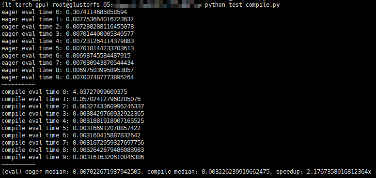
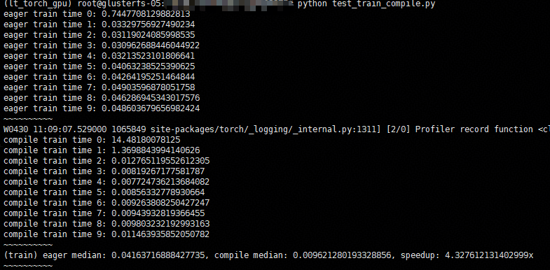
torch.compile第一次迭代耗时较长，因为它必须编译模型，但在随后的迭代中，与 eager 相比，速度明显加快

使用torch.compile 优化后的模型运行速度显著提升。速度提升主要来自于降低 Python 开销和减少 GPU 读写操作，因此观察到的速度提升幅度可能因模型架构和批次大小等因素而异。例如，如果模型架构简单但数据量庞大，那么瓶颈就在于 GPU 计算，此时观察到的速度提升可能并不明显

演示训练

import numpy as np

model = init_model()
opt = torch.optim.Adam(model.parameters())


def train(mod, data):
    opt.zero_grad(True)
    pred = mod(data[0])
    loss = torch.nn.CrossEntropyLoss()(pred, data[1])
    loss.backward()
    opt.step()


eager_times = []
for i in range(N_ITERS):
    inp = generate_data(16)
    _, eager_time = timed(lambda: train(model, inp))
    eager_times.append(eager_time)
    print(f"eager train time {i}: {eager_time}")
print("~" * 10)

model = init_model()
opt = torch.optim.Adam(model.parameters())

# Note that because we are compiling a regular Python function, we do not
# call any .compile() method.
train_opt = torch.compile(train, mode="reduce-overhead")

compile_times = []
for i in range(N_ITERS):
    inp = generate_data(16)
    _, compile_time = timed(lambda: train_opt(model, inp))
    compile_times.append(compile_time)
    print(f"compile train time {i}: {compile_time}")
print("~" * 10)

eager_med = np.median(eager_times)
compile_med = np.median(compile_times)
speedup = eager_med / compile_med
assert speedup > 1
print(
    f"(train) eager median: {eager_med}, compile median: {compile_med}, speedup: {speedup}x"
)
print("~" * 10)

输出：