文章MSM_metagenomics（三）：Alpha多样性分析

欢迎大家关注全网生信学习者系列：

WX公zhong号：生信学习者
Xiao hong书：生信学习者
知hu：生信学习者
CDSN：生信学习者2

介绍

本教程使用基于R的函数来估计微生物群落的香农指数和丰富度，使用MetaPhlAn profile数据。估计结果进一步进行了可视化，并与元数据关联，以测试统计显著性。

数据

大家通过以下链接下载数据：

百度网盘链接：https://pan.baidu.com/s/1f1SyyvRfpNVO3sLYEblz1A
提取码: 请关注WX公zhong号_生信学习者_后台发送 复现msm 获取提取码

R 包

Alpha diversity estimation and visualization

使用alpha_diversity_funcs.R计算alpha多样性和可视化。

代码

r 复制代码

SE_converter <- function(md_rows, tax_starting_row, mpa_md) {
    # SE_converter function is to convery metadata-wedged mpa table into SummarisedExperiment structure.
    # md_rows: a vector specifying the range of rows indicating metadata.
    # tax_starting_row: an interger corresponding to the row where taxonomic abundances start.
    # mpa_md: a metaphlan table wedged with metadata, in the form of dataframe.
    
    md_df <- mpa_md[md_rows,] # extract metadata part from mpa_md table
    tax_df <- mpa_md[tax_starting_row: nrow(mpa_md),] # extract taxonomic abundances part from mpa_md table
    
    ### convert md_df to a form compatible with SummarisedExperiment ### 
    SE_md_df <- md_df[, -1]
    rownames(SE_md_df) <- md_df[, 1]
    SE_md_df <- t(SE_md_df)
    ### convert md_df to a form compatible with SummarisedExperiment ###
    
    ### prep relab values in a form compatible with SummarisedExperiment ###
    SE_relab_df <- tax_df[, -1]
    rownames(SE_relab_df) <- tax_df[, 1]
    col_names <- colnames(SE_relab_df)
    SE_relab_df[, col_names] <- apply(SE_relab_df[, col_names], 2, function(x) as.numeric(as.character(x)))
    ### prep relab values in a form compatible with SummarisedExperiment ###

    SE_tax_df <- tax_df[, 1:2]
    rownames(SE_tax_df) <- tax_df[, 1]
    SE_tax_df <- SE_tax_df[-2]
    colnames(SE_tax_df) <- c("species")
    
    SE_data <- SummarizedExperiment::SummarizedExperiment(assays = list(relative_abundance = SE_relab_df),
                                         colData = SE_md_df,
                                         rowData = SE_tax_df)

    SE_data
}

est_alpha_diversity <- function(se_data) {
    # This function is to estimate alpha diversity (shannon index and richness) of a microbiome and output results in dataframe.
    # se_data: the SummarizedExperiment data structure containing metadata and abundance values.
    se_data <- se_data |>
        mia::estimateRichness(abund_values = "relative_abundance", index = "observed")
    se_data <- se_data |>
        mia::estimateDiversity(abund_values = "relative_abundance", index = "shannon")
    se_alpha_div <- data.frame(SummarizedExperiment::colData(se_data))
    se_alpha_div
}

make_boxplot <- function(df, xlabel, ylabel, font_size = 11, 
                         jitter_width = 0.2, dot_size = 1, 
                         font_style = "Arial", stats = TRUE, pal = NULL) {
    
    # This function is to create a boxplot using categorical data.
    # df: The dataframe containing microbiome alpha diversities, e.g. `shannon` and `observed` with categorical metadata.
    # xlabel: the column name one will put along x-axis.
    # ylabel: the index estimate one will put along y-axis.
    # font_size: the font size, default: [11]
    # jitter_width: the jitter width, default: [0.2]
    # dot_size: the dot size inside the boxplot, default: [1]
    # font_style: the font style, default: `Arial`
    # pal: a list of color codes for pallete, e.g. c(#888888, #eb2525). The order corresponds the column order of boxplot.
    # stats: wilcox rank-sum test. default: TRUE
    if (stats) {
          nr_group = length(unique(df[, xlabel])) # get the number of groups
          if (nr_group == 2) {
              group_pair = list(unique(df[, xlabel]))
              ggpubr::ggboxplot(data = df, x = xlabel, y = ylabel, color = xlabel,
              palette = pal, ylab = ylabel, xlab = xlabel,
              add = "jitter", add.params = list(size = dot_size, jitter = jitter_width)) +
              ggpubr::stat_compare_means(comparisons = group_pair, exact = T, alternative = "less") +
              ggplot2::stat_summary(fun.data = function(x) data.frame(y = max(df[, ylabel]), 
                  label = paste("Mean=",mean(x))), geom="text") +
              ggplot2::theme(text = ggplot2::element_text(size = font_size, family = font_style))
           } else {
              group_pairs = my_combn(unique((df[, xlabel])))
              ggpubr::ggboxplot(data = df, x = xlabel, y = ylabel, color = xlabel,
              palette = pal, ylab = ylabel, xlab = xlabel,
              add = "jitter", add.params = list(size = dot_size, jitter = jitter_width)) +
              ggpubr::stat_compare_means() + 
              ggpubr::stat_compare_means(comparisons = group_pairs, exact = T, alternative = "greater") +
              ggplot2::stat_summary(fun.data = function(x) data.frame(y= max(df[, ylabel]), 
              label = paste("Mean=",mean(x))), geom="text") +
              ggplot2::theme(text = ggplot2::element_text(size = font_size, family = font_style))
           }
    } else {
        ggpubr::ggboxplot(data = df, x = xlabel, y = ylabel, color = xlabel,
        palette = pal, ylab = ylabel, xlab = xlabel,
        add = "jitter", add.params = list(size = dot_size, jitter = jitter_width)) +
        ggplot2::theme(text = ggplot2::element_text(size = font_size, family = font_style))
    }
}

my_combn <- function(x) {
  combs <- list()
  comb_matrix <- combn(x, 2)
  for (i in 1: ncol(comb_matrix)) {
    combs[[i]]  <- comb_matrix[,i]
  }
  combs
}

felm_fixed <- function(data_frame, f_factors, t_factor, measure) {
  # This function is to perform fixed effect linear modeling
  # data_frame: a dataframe containing measures and corresponding effects  
  # f_factors: a vector of header names in the dataframe which represent fixed effects
  # t_factors: test factor name in the form of string
  # measure: the measured values in column, e.g., shannon or richness
#   all_factors <- c(t_factor, f_factors)
#   for (i in all_factors) {
#     vars <- unique(data_frame[, i])
#     lookup <- setNames(seq_along(vars) -1, vars)
#     data_frame[, i] <- lookup[data_frame[, i]]
#   }
#   View(data_frame)
  str1 <- paste0(c(t_factor, paste0(f_factors, collapse = " + ")), collapse = " + ")
  str2 <- paste0(c(measure, str1), collapse = " ~ ")
  felm_stats <- lfe::felm(eval(parse(text = str2)), data = data_frame)
  felm_stats
}

加载一个包含元数据和分类群丰度的合并MetaPhlAn profile文件

r 复制代码

mpa_df <- data.frame(read.csv("./data/merged_abundance_table_species_sgb_md.tsv", header = TRUE, sep = "\t"))

sample	P057	P054	P052	...	P049
sexual_orientation	MSM	MSM	MSM	...	Non-MSM
HIV_status	negative	positive	positive	...	negative
ethnicity	Caucasian	Caucasian	Caucasian	...	Caucasian
antibiotics_6month	Yes	No	No	...	No
BMI_kg_m2_WHO	ObeseClassI	Overweight	Normal	...	Overweight
Methanomassiliicoccales_archaeon	0.0	0.0	0.0	...	0.01322
...	...	...	...	...	...
Methanobrevibacter_smithii	0.0	0.0	0.0	...	0.19154

接下来，我们将数据框转换为SummarizedExperiment数据结构，以便使用SE_converter函数继续分析，该函数需要指定三个参数：

md_rows: a vector specifying the range of rows indicating metadata. Note: 1-based.
tax_starting_row: an interger corresponding to the row where taxonomic abundances start.
mpa_md: a metaphlan table wedged with metadata, in the form of dataframe.

r 复制代码

SE <- SE_converter(md_rows = 1:5,
                   tax_starting_row = 6, 
                   mpa_md = mpa_df)
                   
SE                   

class: SummarizedExperiment
dim: 1676 139
metadata(0):
assays(1): relative_abundance
rownames(1676): Methanomassiliicoccales_archaeon|t__SGB376
  GGB1567_SGB2154|t__SGB2154 ... Entamoeba_dispar|t__EUK46681
  Blastocystis_sp_subtype_1|t__EUK944036
rowData names(1): species
colnames(139): P057 P054 ... KHK16 KHK11
colData names(5): sexual_orientation HIV_status ethnicity
  antibiotics_6month BMI_kg_m2_WHO

接下来，我们可以使用est_alpha_diversity函数来估计每个宏基因组样本的香农指数和丰富度。

r 复制代码

alpha_df <- est_alpha_diversity(se_data = SE)
alpha_df

	sexual_orientation	HIV_status	ethnicity	antibiotics_6month	BMI_kg_m2_WHO	observed	shannon
P057	MSM	negative	Caucasian	Yes	ObeseClassI	134	3.1847
P054	MSM	positive	Caucasian	No	Overweight	141	2.1197
...	...	...	...	...	...	...	...
P052	MSM	positive	Caucasian	No	Normal	152	2.5273

为了比较不同组之间的alpha多样性差异，我们可以使用make_boxplot函数，并使用参数：

df: The dataframe containing microbiome alpha diversities, e.g. shannon and observed with categorical metadata.
xlabel: the column name one will put along x-axis.
ylabel: the index estimate one will put along y-axis.
font_size: the font size, default: [11]
jitter_width: the jitter width, default: [0.2]
dot_size: the dot size inside the boxplot, default: [1]
font_style: the font style, default: Arial
pal: a list of color codes for pallete, e.g. c(#888888, #eb2525). The order corresponds the column order of boxplot.
stats: wilcox rank-sum test. default: TRUE

r 复制代码

shannon <- make_boxplot(df = alpha_df,
                         xlabel = "sexual_orientation",
                         ylabel = "shannon",
                         stats = TRUE,
                         pal = c("#888888", "#eb2525"))

richness <- make_boxplot(df = alpha_df,
                          xlabel = "sexual_orientation", 
                          ylabel = "observed",
                          stats = TRUE,
                          pal = c("#888888", "#eb2525"))
multi_plot <- ggpubr::ggarrange(shannon, richness, ncol = 2)
ggplot2::ggsave(file = "shannon_richness.svg", plot = multi_plot, width = 4, height = 5)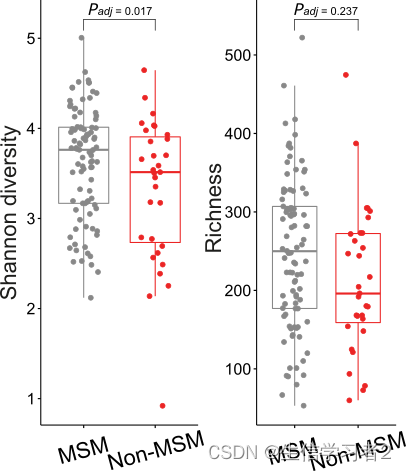

通过固定效应线性模型估计关联的显著性

在宏基因组分析中，除了感兴趣的变量（例如性取向）之外，通常还需要处理多个变量（例如HIV感染和抗生素使用）。因此，在测试微生物群落矩阵（例如香农指数或丰富度）与感兴趣的变量（例如性取向）之间的关联时，控制这些混杂效应非常重要。在这里，我们使用基于固定效应线性模型的felm_fixed函数，该函数实现在R包lfe 中，以估计微生物群落与感兴趣变量之间的关联显著性，同时控制其他变量的混杂效应。

data_frame: The dataframe containing microbiome alpha diversities, e.g. shannon and observed with multiple variables.
f_factors: A vector of variables representing fixed effects.
t_factor: The variable of interest for testing.
measure: The header indicating microbiome measure, e.g. shannon or richness

r 复制代码

lfe_stats <- felm_fixed(data_frame = alpha_df,
                         f_factors = c(c("HIV_status", "antibiotics_6month")),
                         t_factor = "sexual_orientation",
                         measure = "shannon")
summary(lfe_stats)
Residuals:
    Min      1Q  Median      3Q     Max 
-2.3112 -0.4666  0.1412  0.5200  1.4137 

Coefficients:
                      Estimate Std. Error t value Pr(>|t|)    
(Intercept)            3.62027    0.70476   5.137 9.64e-07 ***
sexual_orientationMSM  0.29175    0.13733   2.125   0.0355 *  
HIV_statuspositive    -0.28400    0.14658  -1.937   0.0548 .  
antibiotics_6monthNo  -0.10405    0.67931  -0.153   0.8785    
antibiotics_6monthYes  0.01197    0.68483   0.017   0.9861    
---
Signif. codes:  0 '***' 0.001 '**' 0.01 '*' 0.05 '.' 0.1 ' ' 1

Residual standard error: 0.6745 on 134 degrees of freedom
Multiple R-squared(full model): 0.07784   Adjusted R-squared: 0.05032 
Multiple R-squared(proj model): 0.07784   Adjusted R-squared: 0.05032 
F-statistic(full model):2.828 on 4 and 134 DF, p-value: 0.02725 
F-statistic(proj model): 2.828 on 4 and 134 DF, p-value: 0.02725