信号的图小波变换（Python）

可以换个空间，从图域的角度进行分析，比如图傅里叶变换，图小波变换等图时频分析方法。图小波阈值降噪的基本思想是通过将时间序列信号转换成路图信号，再利用图小波变换分解成尺度函数系数和一系列对应不同尺度的谱图小波系数，然后设置阈值对图小波系数进行过滤处理，最后对尺度函数系数和滤波后的图小波系数进行图小波逆变换，重构得到降噪信号。

更具体地，图小波变换将路图信号分解成低频分量和高频分量，其中尺度函数系数包含信号的低频近似成分，图小波系数反映信号的高频细节成分。各尺度上的图小波系数在某些特定位置的幅值较大，对应于原始信号的奇变位置和重要信息，而其他大部分位置的幅值较小，对应于噪声干扰成分。噪声对应的图小波系数在每个尺度上的分布较均匀，且幅值随着尺度的减小而逐渐减小。因此，通常的降噪方法是设置一个合适的临界阈值ρ，并结合阈值函数对系数进行滤波。当图小波系数小于阈值ρ时，认为此系数主要由噪声引起，则将其置为零进行消除；当图小波系数大于或等于阈值ρ时，认为此系数主要由信号引起，则予以保留或进行收缩，从而得到估计谱图小波系数。最后，对所有剩余系数进行重构即可获得降噪信号。

import sys
import os
sys.path.append("src")


import numpy as np
import networkx as nx
import matplotlib.pyplot as plt
import wavelet_transform as wt
from pygsp import graphs
from time import time
if not os.path.exists("figs"):
    os.makedirs("figs")
def plot_graph_signal(
        G,
        signal,
        pos = None,
        vmin = None,
        vmax = None,
        ax = None,
        fig = None,
        colorbar = True,
        colorbar_label = "Values",
    ):
    if ax is None:
        fig, ax = plt.subplots(figsize = (4, 4))
    
    vmin = np.min(signal) if vmin is None else vmin
    vmax = np.max(signal) if vmax is None else vmax
   
    pathcollection = nx.draw_networkx_nodes(
        G, 
        pos, 
        node_color=signal,
        cmap=plt.cm.magma, 
        node_size=50,
        edgecolors="#909090",
        ax = ax,
        vmin = vmin,
        vmax = vmax
    )
    nx.draw_networkx_edges(
        G, 
        pos,
        edge_color="#909090", 
        ax = ax
    )
    
    ax.axis("off")
    if colorbar:
        fig.colorbar(pathcollection, ax = ax, label = colorbar_label)
        ax.figure.axes[-1].yaxis.label.set_size(14)
    return ax

Creating Graph

def create_grid_graph(size = 17):
    g = nx.grid_2d_graph(size, size)
    nodes = list(g.nodes)
    pos = {node: node for node in g.nodes}
    pos = np.array(list(pos.values()))
    for node in nodes:
        # get node position
        node_pos = np.array(node)
        # get all nodes closest than \sqrt 2
        distances = np.linalg.norm(pos - node_pos, axis = 1)
        idx_close = (distances < 2) & (distances != 0) & (distances != 1)
        close_node = np.random.choice(np.where(idx_close)[0])


        # select a random close node
        n1 = close_node


        # add edge
        g.add_edge(node, tuple(nodes[n1]))


    return g
# create 2D grid graph
np.random.seed(1)
g = create_grid_graph(17)




adj_matrix = nx.adjacency_matrix(g).todense()


# darw nodes by position
pos = {node: node for node in g.nodes}
pos = np.array(list(pos.values()))
# add random noise
#pos = pos + np.random.normal(0, 0.15, pos.shape)
pos = {node: pos[i] for i, node in enumerate(g.nodes)}
nx.draw(g, pos, node_size = 75, node_color = "#034e7b", edgecolors = "black", width = 1)
plt.axis("off")
plt.title("Grid Graph")
plt.savefig("figs/grid_graph.pdf", dpi = 300)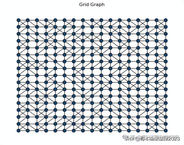

Fourier Transform

G = graphs.Graph(adj_matrix)
G.compute_fourier_basis()
fig, ax = plt.subplots(nrows = 1, ncols = 1, figsize = (6, 4))
ax.hist(G.e, bins = 40)
ax.set_title("Distribution of Eigenvalues", fontsize = 16)
ax.set_xlabel("Eigenvalue", fontsize = 14)
ax.set_ylabel("Frequency", fontsize = 14)
plt.savefig("figs/eigenvalues_dist.svg", dpi = 300)
plt.show()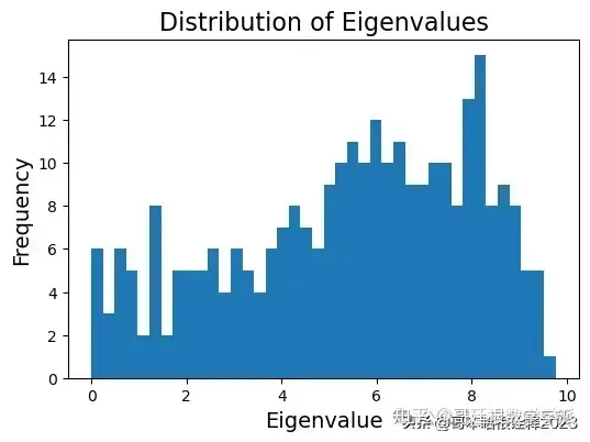

fig, axs = plt.subplots(nrows = 1, ncols = 3, figsize = (14, 4))
for i, idx in enumerate([4, 9, 14]):
    plot_graph_signal(
        g, 
        G.U[:, idx], 
        pos = pos, 
        ax = axs[i],
        vmin = -0.15,
        vmax = 0.10,
        fig=fig
    )
    axs[i].set_title(f"{idx+1}-th Eigenvector", fontsize = 14)
   
plt.suptitle("Eigenvectors of Graph", fontsize = 16)
plt.tight_layout()
plt.savefig("figs/eigenvectors.svg", dpi = 300)
plt.show()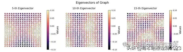

simple_signal = np.zeros((2, 17, 17))


for i in range(17):
    for j in range(17):
        simple_signal[0, i, j] = (i + j)**2 / (34)**2
        simple_signal[1, i, j] = np.sin(i + j)


fig, axs = plt.subplots(nrows = 1, ncols = 2, figsize = (10, 4))
plot_graph_signal(
    g, 
    simple_signal[0].flatten(), 
    pos = pos, 
    ax = axs[0],
    vmin = -1,
    vmax = 1,
    fig=fig
)


plot_graph_signal(
    g, 
    simple_signal[1].flatten(), 
    pos = pos, 
    ax = axs[1],
    vmin = -1,
    vmax = 1,
    fig=fig,
    colorbar_label="Signal Value"
)


axs[0].set_title("Simple Signal 1", fontsize = 14)
axs[1].set_title("Simple Signal 2", fontsize = 14)


plt.suptitle("Fourier Transform of Two Signals", fontsize = 16)
plt.tight_layout()
plt.savefig("figs/simple_signals.svg", dpi = 300)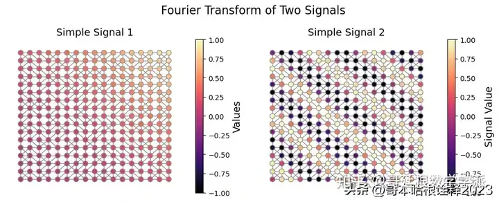

transformed_signal = [G.gft(signal.flatten()) for signal in simple_signal]


fig, axs = plt.subplots(nrows = 1, ncols = 2, figsize = (10, 4))


for i in range(2):
    axs[i].plot(G.e, transformed_signal[i])
    axs[i].set_ylabel("$\hat f(\lambda)$", fontsize = 14)
    axs[i].set_xlabel("$\lambda$", fontsize = 14)
    axs[i].set_title(f"Signal {i+1} Fourier Transform", fontsize = 14)
#plt.suptitle("Graph Fourier Transform of Signals")
plt.tight_layout()
plt.savefig("figs/fourier_transform.svg", dpi = 300)
plt.show()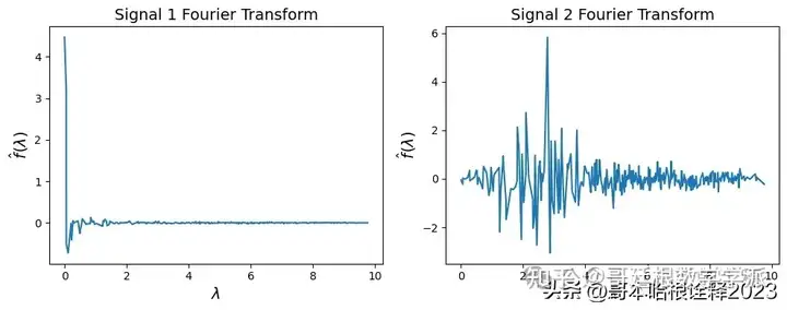

Graph Wavelet Transform

signal = np.random.normal(0, 0.25, (17, 17)) + 3


for i in range(17):
    for j in range(17):
        if (i - 8)**2 + (j - 8)**2 <= 25:
            signal[i, j] += 3


signal = signal.flatten()


adj_matrix = np.array(nx.adjacency_matrix(g).todense())
wav = wt.WaveletTransform(
    adj_matrix = adj_matrix,
    n_timestamps=1,
    method = "exact_fast",
    scaling_function=False,
    n_filters=4
)
coeffs = wav.transform(signal.reshape(-1, 1))
coeffs_ = coeffs.reshape(17, 17, 4)
selected_nodes = [
    [11, 11],
    [12, 12],
    [15, 15],
]
selected_nodes_idx = [ x + y * 17 for (x, y) in selected_nodes]
fig = plt.figure(figsize = (6, 4))
pathcollection = nx.draw_networkx_nodes(
    g, 
    pos, 
    node_color=signal, 
    cmap=plt.cm.magma, 
    node_size=[100 if i in selected_nodes_idx else 50 for i in range(len(pos))],
    edgecolors=["#e7298a" if i in selected_nodes_idx else "#909090" for i in range(len(pos))],
    #vmin = 1
)
nx.draw_networkx_edges(g, pos, edge_color="#909090")
plt.colorbar(pathcollection, label = "Signal")
plt.title("Graph with Signal")
plt.axis("off")
plt.savefig("figs/graph_with_signal.svg", dpi = 300)
plt.show()






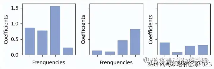
fig, axs = plt.subplots(nrows = 1, ncols = 3, figsize =(6, 2), sharex = True, sharey = True)


for i in range(3):
    c = np.abs(coeffs_[selected_nodes[i][0], selected_nodes[i][1], :])
    axs[i].bar(range(4), c, color = "#8da0cb")


    axs[i].set_xticks(range(4), labels = ["" for _ in range(4)])
    #axs[i].set_yticks([])
    axs[i].set_xlabel("Frenquencies")
    axs[i].set_ylabel("Coefficients")


plt.tight_layout()
plt.savefig("figs/coefs.svg", dpi = 300)
plt.show()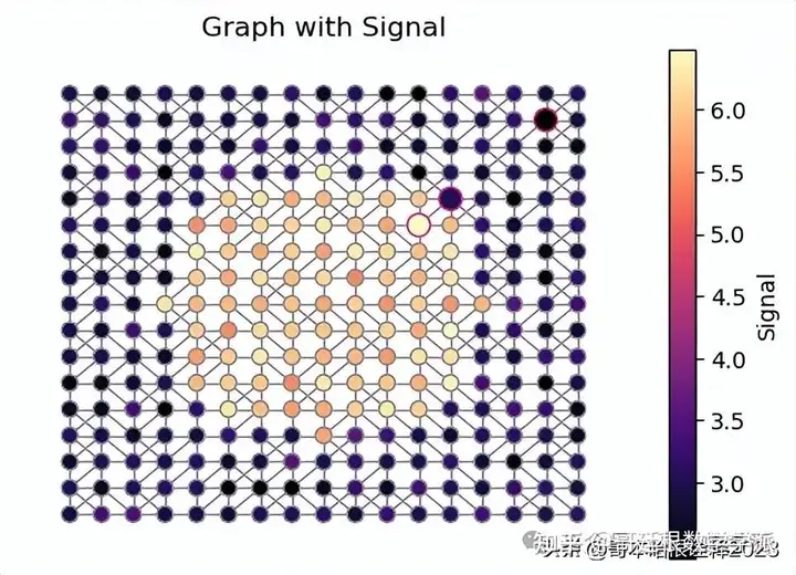

Fast Computation

graph_sizes = [5, 10, 15, 20, 25, 30]
exact_time = []
cheb_time = []
cheb_error = []


for n_g in graph_sizes:
    signal = np.random.random((n_g**2, 20))
    g = create_grid_graph(n_g)
    adj_matrix = nx.adjacency_matrix(g).todense()
    times_ = []
    for _ in range(10):
        start = time()
        wav = wt.WaveletTransform(
            adj_matrix = adj_matrix,
            n_timestamps=20,
            method = "exact_low_memory",
            scaling_function=False,
            n_filters=4
        )
        coeffs_exact = wav.transform(signal)
        end = time()
        times_.append(end - start)
    exact_time.append(np.mean(times_))


    times_ = []
    for _ in range(10):
        start = time()
        wav = wt.WaveletTransform(
            adj_matrix = adj_matrix,
            n_timestamps=20,
            method = "chebyshev",
            scaling_function=False,
            n_filters=4
        )
        coeffs_cheb = wav.transform(signal)
        end = time()
        times_.append(end - start)
    cheb_time.append(np.mean(times_))
    cheb_error.append(np.mean(np.abs(coeffs_exact - coeffs_cheb) / np.abs(coeffs_exact)))
fig, axs = plt.subplots(nrows = 1, ncols = 2, figsize = (7, 2.5))
axs[0].plot(graph_sizes, exact_time, label = "Exact")
axs[0].plot(graph_sizes, cheb_time, label = "Chebyshev")


axs[1].plot(graph_sizes, cheb_error, label = "Chebyshev")
for i in range(2):
    axs[i].set_xlabel("Graph Size")
    axs[i].set_xticks(graph_sizes, labels = [int(x*x*20) for x in graph_sizes])
axs[0].set_ylabel("Time (s)")
axs[0].legend()
axs[1].set_ylabel("Mean Absolute\nPercentage Error")
plt.suptitle("Time and Error of Exact and Chebyshev Methods")
plt.tight_layout()
plt.savefig("figs/time_error.pdf", dpi = 300)
plt.show()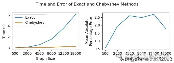

n_order = [10, 20, 30, 40, 50]
cheb_time = []
cheb_error = []


g = create_grid_graph(17)
adj_matrix = nx.adjacency_matrix(g).todense()
signal = np.random.random((17**2, 20))
wav = wt.WaveletTransform(
    adj_matrix = adj_matrix,
    n_timestamps=20,
    method = "exact_low_memory",
    scaling_function=False,
    n_filters=4
)
coeffs_exact = wav.transform(signal)


for order in n_order:
    times_ = []
    for i in range(10):
        start = time()
        wav = wt.WaveletTransform(
            adj_matrix = adj_matrix,
            n_timestamps=20,
            method = "chebyshev",
            scaling_function=False,
            n_filters=4,
            order_chebyshev=order,
        )
        coeffs_cheb = wav.transform(signal)
        end = time()
        times_.append(end - start)
    cheb_time.append(np.mean(times_))
    # append MAPE
    cheb_error.append(np.mean(np.abs(coeffs_exact - coeffs_cheb) / np.abs(coeffs_exact)))
fig, axs = plt.subplots(nrows = 1, ncols = 2, figsize = (7, 2.5))


axs[0].plot(n_order, cheb_time, label = "Chebyshev")
axs[1].plot(n_order, cheb_error, label = "Chebyshev")


for i in range(2):
    axs[i].set_xlabel("Chebyshev Order")
    axs[i].set_xticks(n_order)
axs[0].set_ylabel("Time (s)")
axs[1].set_ylabel("Mean Absolute\nPercentage Error")
axs[1].set_yscale("log")
plt.suptitle("Time and Error of Chebyshev Method")
plt.tight_layout()
plt.savefig("figs/time_error_cheb_order.pdf", dpi = 300)
plt.show()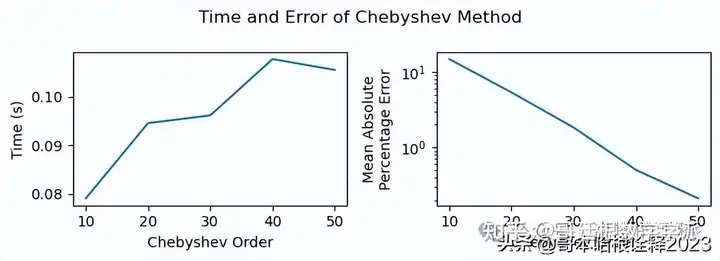

擅长领域：现代信号处理，机器学习，深度学习，数字孪生，时间序列分析，设备缺陷检测、设备异常检测、设备智能故障诊断与健康管理PHM等。
知乎学术咨询：https://www.zhihu.com/consult/people/792359672131756032?isMe=1
擅长领域：现代信号处理，机器学习，深度学习，数字孪生，时间序列分析，设备缺陷检测、设备异常检测、设备智能故障诊断与健康管理PHM等。

擅长领域：现代信号处理，机器学习，深度学习，数字孪生，时间序列分析，设备缺陷检测、设备异常检测、设备智能故障诊断与健康管理PHM等。