Method 1
# Method 1: create_sequences function
def create_sequences_meth1(data, target_col, sequence_length=10):
sequences = []
targets = []
for i in range(len(data) - sequence_length):
seq = data[i:i + sequence_length].drop(columns=[target_col]).values
label = data.iloc[i + sequence_length][target_col]
sequences.append(seq)
targets.append(label)
return np.array(sequences), np.array(targets)
scaler_meth1 = MinMaxScaler()
scaled_df_meth1 = pd.DataFrame(scaler_meth1.fit_transform(df), columns=df.columns)
sequence_length = 100
num_features = len(df.columns)
X_meth1, y_meth1 = create_sequences_meth1(scaled_df_meth1, target_col='RH', sequence_length=sequence_length)
split_ratio = 0.8
split_index = int(len(X_meth1) * split_ratio)
X_train_meth1, X_test_meth1 = X_meth1[:split_index], X_meth1[split_index:]
y_train_meth1, y_test_meth1 = y_meth1[:split_index], y_meth1[split_index:]
X_train_meth1 = X_train_meth1.reshape((X_train_meth1.shape[0], X_train_meth1.shape[1], X_train_meth1.shape[2]))
X_test_meth1 = X_test_meth1.reshape((X_test_meth1.shape[0], X_test_meth1.shape[1], X_test_meth1.shape[2]))
optimizer_meth1 = Adam(lr=0.001)
model_meth1 = Sequential()
model_meth1.add(LSTM(32, return_sequences=True, input_shape=(X_train_meth1.shape[1], X_train_meth1.shape[2])))
model_meth1.add(Dropout(0.2))
model_meth1.add(LSTM(32))
model_meth1.add(Dropout(0.2))
model_meth1.add(Dense(1))
model_meth1.compile(loss='mse', optimizer=optimizer_meth1, metrics=['mse'])
early_stopping_meth1 = EarlyStopping(monitor='val_loss', patience=10, restore_best_weights=True)
history_meth1 = model_meth1.fit(X_train_meth1, y_train_meth1, epochs=200, batch_size=50,
validation_data=(X_test_meth1, y_test_meth1), verbose=0,
callbacks=[early_stopping_meth1], shuffle=False)
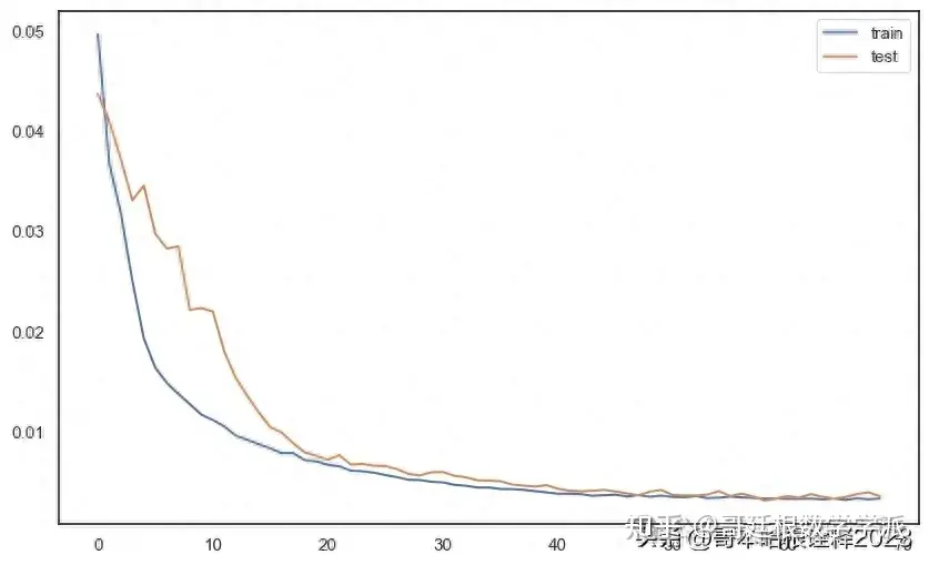
plt.figure(figsize=(10, 6))
plt.plot(history_meth1.history['loss'], label='train')
plt.plot(history_meth1.history['val_loss'], label='test')
plt.legend()
plt.show()
predictions_meth1 = model_meth1.predict(X_test_meth1)
X_test_reshaped_meth1 = X_test_meth1.reshape((X_test_meth1.shape[0], X_test_meth1.shape[1] * X_test_meth1.shape[2]))
inv_preds_meth1 = np.concatenate((predictions_meth1, X_test_reshaped_meth1[:, -(num_features - 1):]), axis=1)
inv_preds_meth1 = scaler_meth1.inverse_transform(inv_preds_meth1)
inv_preds_meth1 = inv_preds_meth1[:, 0]
y_test_reshaped_meth1 = y_test_meth1.reshape((len(y_test_meth1), 1))
inv_actual_y_meth1 = np.concatenate((y_test_reshaped_meth1, X_test_reshaped_meth1[:, -(num_features - 1):]), axis=1)
inv_actual_y_meth1 = scaler_meth1.inverse_transform(inv_actual_y_meth1)
inv_actual_y_meth1 = inv_actual_y_meth1[:, 0]
print("Predictions Method 1:", inv_preds_meth1)
print("Actual values Method 1:", inv_actual_y_meth1)
58/58 [==============================] - 1s 13ms/step
Predictions Method 1: [20.72510315 13.99930025 11.20439576 ... 2.88401567 0.74950135
-0.53083279]
Actual values Method 1: [16.40754717 13.01509434 12.19622642 ... 3.42264151 0.61509434
0.38113208]
# Evaluate Method 1
mse_meth1 = mean_squared_error(inv_actual_y_meth1, inv_preds_meth1)
rmse_meth1 = np.sqrt(mse_meth1)
r2_meth1 = r2_score(inv_actual_y_meth1, inv_preds_meth1)
mae_meth1 = mean_absolute_error(inv_actual_y_meth1, inv_preds_meth1)
print(f'Method 1 - Mean Squared Error (MSE): {mse_meth1}')
print(f'Method 1 - Root Mean Squared Error (RMSE): {rmse_meth1}')
print(f'Method 1 - R-squared (R2): {r2_meth1}')
print(f'Method 1 - Mean Absolute Error (MAE): {mae_meth1}')
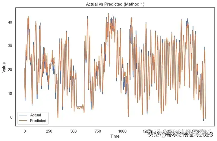
Method 1 - Mean Squared Error (MSE): 6.851774623441025
Method 1 - Root Mean Squared Error (RMSE): 2.617589468087199
Method 1 - R-squared (R2): 0.9328422940803206
Method 1 - Mean Absolute Error (MAE): 1.8842330539870726
# Visualize actual vs predicted for Method 1
plt.figure(figsize=(10, 6))
plt.plot(inv_actual_y_meth1, label='Actual')
plt.plot(inv_preds_meth1, label='Predicted')
plt.title('Actual vs Predicted (Method 1)')
plt.xlabel('Time')
plt.ylabel('Value')
plt.legend()
plt.show()
Method 2
# Method 2: making_supervised function
def making_supervised_meth2(data, number_input=1, number_output=1, dropnan=True):
    number_variables = 1 if type(data) is list else data.shape[1]
    df = pd.DataFrame(data)
    cols, names = list(), list()
    for i in range(number_input, 0, -1):
        cols.append(df.shift(i))
        names += [('var%d(t-%d)' % (j+1, i)) for j in range(number_variables)]
    for i in range(0, number_output):
        cols.append(df.shift(-i))
        if i == 0:
            names += [('var%d(t)' % (j+1)) for j in range(number_variables)]
        else:
            names += [('var%d(t+%d)' % (j+1, i)) for j in range(number_variables)]
    agg = pd.concat(cols, axis=1)
    agg.columns = names
    if dropnan:
        agg.dropna(inplace=True)
    return agg
scaler_meth2 = MinMaxScaler()
scaled_values_meth2 = scaler_meth2.fit_transform(df.values)
scaled_df_meth2 = pd.DataFrame(scaled_values_meth2, columns=df.columns)
number_input = 100
number_output = 1
reframed_meth2 = making_supervised_meth2(scaled_df_meth2, number_input, number_output)
target_col_index = len(df.columns) * number_input


drop_columns = [i for i in range(target_col_index, reframed_meth2.shape[1]) if (i - target_col_index) % len(df.columns) != len(df.columns) - 1]
reframed_meth2.drop(reframed_meth2.columns[drop_columns], axis=1, inplace=True)
values_meth2 = reframed_meth2.values
n_train_hours = int(len(values_meth2) * 0.8)
train_meth2 = values_meth2[:n_train_hours, :]
test_meth2 = values_meth2[n_train_hours:, :]


X_train_meth2, y_train_meth2 = train_meth2[:, :-1], train_meth2[:, -1]
X_test_meth2, y_test_meth2 = test_meth2[:, :-1], test_meth2[:, -1]


X_train_meth2 = X_train_meth2.reshape((X_train_meth2.shape[0], number_input, len(df.columns)))
X_test_meth2 = X_test_meth2.reshape((X_test_meth2.shape[0], number_input, len(df.columns)))
optimizer_meth2 = Adam(lr=0.001)
model_meth2 = Sequential()
model_meth2.add(LSTM(64, return_sequences=True, input_shape=(X_train_meth2.shape[1], X_train_meth2.shape[2])))
model_meth2.add(Dropout(0.2))
model_meth2.add(LSTM(64))
model_meth2.add(Dropout(0.2))
model_meth2.add(Dense(1))
model_meth2.compile(loss='mse', optimizer=optimizer_meth2, metrics=['mse'])


early_stopping_meth2 = EarlyStopping(monitor='val_loss', patience=10, restore_best_weights=True)
history_meth2 = model_meth2.fit(X_train_meth2, y_train_meth2, epochs=200, batch_size=50,
                                validation_data=(X_test_meth2, y_test_meth2), verbose=0,
                                callbacks=[early_stopping_meth2], shuffle=False)
plt.figure(figsize=(10, 6))
plt.plot(history_meth2.history['loss'], label='train')
plt.plot(history_meth2.history['val_loss'], label='test')
plt.legend()
plt.show()

predictions_meth2 = model_meth2.predict(X_test_meth2)
X_test_reshaped_meth2 = X_test_meth2.reshape((X_test_meth2.shape[0], number_input * len(df.columns)))
inv_preds_meth2 = np.concatenate((predictions_meth2, X_test_reshaped_meth2[:, -(len(df.columns) - 1):]), axis=1)
inv_preds_meth2 = scaler_meth2.inverse_transform(inv_preds_meth2)
inv_preds_meth2 = inv_preds_meth2[:, 0]
y_test_reshaped_meth2 = y_test_meth2.reshape((len(y_test_meth2), 1))
inv_actual_y_meth2 = np.concatenate((y_test_reshaped_meth2, X_test_reshaped_meth2[:, -(len(df.columns) - 1):]), axis=1)
inv_actual_y_meth2 = scaler_meth2.inverse_transform(inv_actual_y_meth2)
inv_actual_y_meth2 = inv_actual_y_meth2[:, 0]
print("Predictions Method 2:", inv_preds_meth2)
print("Actual values Method 2:", inv_actual_y_meth2)
58/58 [==============================] - 2s 20ms/step
Predictions Method 2: [20.05376787 13.37555639 11.81537217 ... 4.66319288 1.91325717
-0.3942143 ]
Actual values Method 2: [16.40754717 13.01509434 12.19622642 ... 3.42264151 0.61509434
0.38113208]
# Evaluate Method 2
mse_meth2 = mean_squared_error(inv_actual_y_meth2, inv_preds_meth2)
rmse_meth2 = np.sqrt(mse_meth2)
r2_meth2 = r2_score(inv_actual_y_meth2, inv_preds_meth2)
mae_meth2 = mean_absolute_error(inv_actual_y_meth2, inv_preds_meth2)
print(f'Method 2 - Mean Squared Error (MSE): {mse_meth2}')
print(f'Method 2 - Root Mean Squared Error (RMSE): {rmse_meth2}')
print(f'Method 2 - R-squared (R2): {r2_meth2}')
print(f'Method 2 - Mean Absolute Error (MAE): {mae_meth2}')
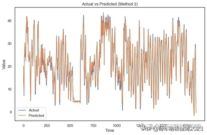
Method 2 - Mean Squared Error (MSE): 5.7881381678302954
Method 2 - Root Mean Squared Error (RMSE): 2.4058549764751604
Method 2 - R-squared (R2): 0.943267532535622
Method 2 - Mean Absolute Error (MAE): 1.7095511506826195
# Visualize actual vs predicted for Method 2
plt.figure(figsize=(10, 6))
plt.plot(inv_actual_y_meth2, label='Actual')
plt.plot(inv_preds_meth2, label='Predicted')
plt.title('Actual vs Predicted (Method 2)')
plt.xlabel('Time')
plt.ylabel('Value')
plt.legend()
plt.show()
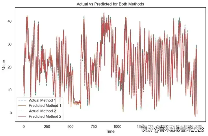
Comparison of Methods
plt.figure(figsize=(10, 6))
plt.plot(inv_actual_y_meth1, label='Actual Method 1', linestyle='dashed')
plt.plot(inv_preds_meth1, label='Predicted Method 1')
plt.plot(inv_actual_y_meth2, label='Actual Method 2', linestyle='dotted')
plt.plot(inv_preds_meth2, label='Predicted Method 2')
plt.title('Actual vs Predicted for Both Methods')
plt.xlabel('Time')
plt.ylabel('Value')
plt.legend()
plt.show()
# Metrics from Method 1
metrics_meth1 = {
    "MSE": mse_meth1,
    "RMSE": rmse_meth1,
    "R2": r2_meth1,
    "MAE": mae_meth1
}


# Metrics from Method 2
metrics_meth2 = {
    "MSE": mse_meth2,
    "RMSE": rmse_meth2,
    "R2": r2_meth2,
    "MAE": mae_meth2
}


# Create DataFrame for comparison
comparison_df = pd.DataFrame([metrics_meth1, metrics_meth2], index=['Method 1', 'Method 2'])


print(comparison_df)
MSE      RMSE        R2       MAE
Method 1  6.851775  2.617589  0.932842  1.884233
Method 2  5.788138  2.405855  0.943268  1.709551

担任《Mechanical System and Signal Processing》审稿专家,担任《中国电机工程学报》,《控制与决策》等EI期刊审稿专家,擅长领域:现代信号处理,机器学习,深度学习,数字孪生,时间序列分析,设备缺陷检测、设备异常检测、设备智能故障诊断与健康管理PHM等。

知乎学术咨询:https://www.zhihu.com/consult/people/792359672131756032?isMe=1