pip install dartsImporting Necessary FrameWorks
import pandas as pd
from darts import TimeSeries
from darts.dataprocessing.transformers import Scaler
from darts.models import TCNModel
from darts import TimeSeries
from darts.ad.utils import (
    eval_metric_from_binary_prediction,
    eval_metric_from_scores,
    show_anomalies_from_scores,
)
from darts.ad import (
    ForecastingAnomalyModel,
    KMeansScorer,
    NormScorer,
    WassersteinScorer,
)
from darts.metrics import mae, rmse
import logging
import torch
import numpy as np
Data Loading and preparation for Training
# Load the data (replace 'train.txt' and 'test.txt' with your actual file names)
train_data = pd.read_csv('ECG5000_TRAIN.txt', delim_whitespace=True, header=None)
test_data = pd.read_csv('ECG5000_TEST.txt', delim_whitespace=True, header=None)


# Check for null values in both datasets
print("Null values in training data:", train_data.isnull().sum().sum())
print("Null values in testing data:", test_data.isnull().sum().sum())
Null values in training data: 0
Null values in testing data: 0
# Merge the datasets row-wise
combined_data = pd.concat([train_data, test_data], axis=0).reset_index(drop=True)


train_final = combined_data[combined_data[0] == 1].reset_index(drop=True)
test_final = combined_data[combined_data[0] != 1].reset_index(drop=True)


# Drop the label column (0th column)
train_final = train_final.drop(columns=[0])
test_final = test_final.drop(columns=[0])


# Convert to TimeSeries objects
series = TimeSeries.from_dataframe(train_final)
test_series = TimeSeries.from_dataframe(test_final)
# anomalies = TimeSeries.from_dataframe(anomalies)


# Manually split the data into train and validation sets (e.g., 80% train, 20% val)
train_size = int(0.8 * len(series))
train_series = series[:train_size]
val_series = series[train_size:]
Data Normalization Using Darts
# Normalize the data using Darts Scaler
scaler = Scaler()
train_series_scaled = scaler.fit_transform(train_series)
val_series_scaled = scaler.transform(val_series)
test_series_scaled = scaler.transform(test_series)
Early Stopping
from pytorch_lightning.callbacks.early_stopping import EarlyStopping


# stop training when validation loss does not decrease more than 0.05 (`min_delta`) over
# a period of 5 epochs (`patience`)
my_stopper = EarlyStopping(
    monitor="val_loss",
    patience=5,
    min_delta=0.05,
    mode='min',
)
# Define and train the TCN model without covariates
model = TCNModel(
    input_chunk_length=30,  # Adjust based on your data
    output_chunk_length=10,  # Adjust based on desired forecast horizon,
    dropout=0.3,               # Dropout rate to prevent overfitting
    weight_norm=True,
    random_state=42,
    pl_trainer_kwargs={"callbacks": [my_stopper]}
)
# Fit the model on the training data
model.fit(series=train_series_scaled, val_series=val_series_scaled, epochs = 30)
TCNModel(output_chunk_shift=0, kernel_size=3, num_filters=3, num_layers=None, dilation_base=2, weight_norm=True, dropout=0.3, input_chunk_length=30, output_chunk_length=10, random_state=42, pl_trainer_kwargs={'callbacks': [<pytorch_lightning.callbacks.early_stopping.EarlyStopping object at 0x7baec921b250>]})
# torch.save(model.state_dict(), 'model.pth')
torch.save(model, 'full_model.pth')
Comparing Actual Vs Prediction For VAL Data
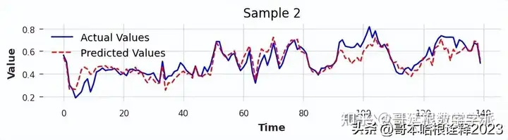
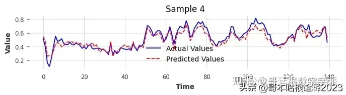
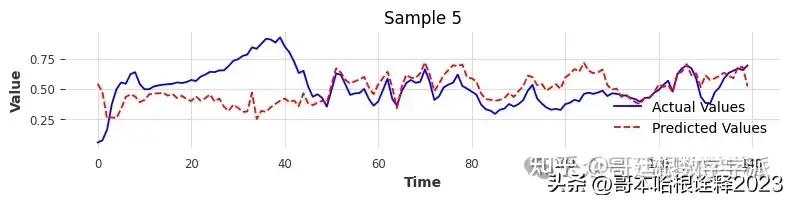
# Number of samples to visualize
num_samples = 5


plt.figure(figsize=(15, num_samples * 5))


for i in range(num_samples):


    val_series_sample = val_series_scaled[i]


    # Predict using the model
    prediction = model.predict(n=len(val_series_sample))


    # Convert the TimeSeries objects to numpy arrays for plotting
    actual_values = val_series_sample.pd_dataframe().values.flatten()
    predicted_values = prediction.pd_dataframe().values.flatten()


    # Plot the results
    plt.figure(figsize=(8,8))
    plt.subplot(num_samples, 1, i + 1)
    plt.plot(actual_values, label='Actual Values', color='blue')
    plt.plot(predicted_values, label='Predicted Values', color='red', linestyle='--')
    plt.title(f'Sample {i + 1}')
    plt.xlabel('Time')
    plt.ylabel('Value')
    plt.legend()
    plt.grid(True)


plt.tight_layout()
plt.show()

Comparing Actual Vs Predicted For Test Data
num_samples = 5


plt.figure(figsize=(15, num_samples * 5))


for i in range(num_samples):
    # Extract the i-th test series
    test_series_sample = test_series_scaled[i]


    # Predict using the model
    prediction = model.predict(n=len(test_series_sample))


    # Convert the TimeSeries objects to numpy arrays for plotting
    actual_values = test_series_sample.pd_dataframe().values.flatten()
    predicted_values = prediction.pd_dataframe().values.flatten()


    # Plot the results
    plt.subplot(num_samples, 1, i + 1)
    plt.plot(actual_values, label='Actual Values', color='blue')
    plt.plot(predicted_values, label='Predicted Values', color='red', linestyle='--')
    plt.title(f'Test Sample {i + 1}')
    plt.xlabel('Time')
    plt.ylabel('Value')
    plt.legend()
    plt.grid(True)


plt.tight_layout()
plt.show()
Checking Val Prediction Error to find Suitable Threshold
# Parameters
chunk_size = 20
num_chunks_divisor = 7


# Initialize lists to store chunk-wise errors and average errors per series
chunk_errors_list = []
average_errors_per_series = []


# Set logging level to suppress PyTorch Lightning outputs
logging.getLogger("pytorch_lightning").setLevel(logging.ERROR)


# Iterate over each validation sample
for val_series in val_series_scaled:
    # Predict using the model
    prediction = model.predict(n=len(val_series))


    # Convert TimeSeries objects to numpy arrays
    actual_values = val_series.pd_dataframe().values.flatten()
    predicted_values = prediction.pd_dataframe().values.flatten()


    # Ensure actual and predicted values have the same length
    if len(actual_values) != len(predicted_values):
        continue  # Skip if lengths do not match


    # Compute average error per chunk
    chunk_errors = []
    num_chunks = len(actual_values) // chunk_size


    for i in range(num_chunks):
        start_idx = i * chunk_size
        end_idx = start_idx + chunk_size
        chunk_actual = actual_values[start_idx:end_idx]
        chunk_predicted = predicted_values[start_idx:end_idx]


        # Calculate error for the chunk
        chunk_error = np.mean(np.abs(chunk_actual - chunk_predicted))
        chunk_errors.append(chunk_error)
        chunk_errors_list.extend(chunk_errors)  # Add chunk errors to the list


    # Calculate average chunk error per series
    average_chunk_error = np.mean(chunk_errors)
    average_error_per_series = average_chunk_error
    average_errors_per_series.append(average_error_per_series)


# Sort chunk errors in descending order
chunk_errors_list_sorted = sorted(chunk_errors_list, reverse=True)


# Plot error vs. series number
plt.figure(figsize=(10, 6))
plt.plot(range(len(average_errors_per_series)), average_errors_per_series, marker='o', linestyle='-', color='blue')
plt.title('Average Error per Series with Threshold')
plt.xlabel('Series Number')
plt.ylabel('Average Error')
plt.legend()
plt.grid(True)
plt.show()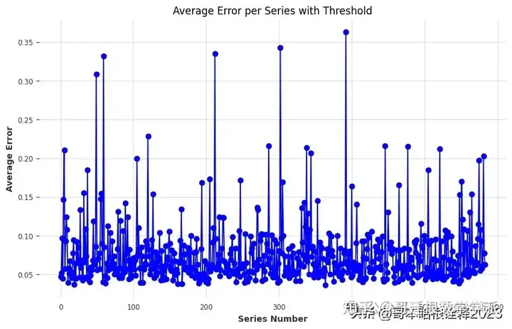
As it can be seen from upper graph, 0.15 is a good option for threshold.
Anomaly Detection Based On Error
chunk_size = 20
error_threshold = 0.15


# Select a random test sample
import random
sample_index = 1000
test_series_sample = test_series_scaled[sample_index]


# Predict using the model
prediction = model.predict(n=len(test_series_sample))


# Convert TimeSeries objects to numpy arrays
actual_values = test_series_sample.pd_dataframe().values.flatten()
predicted_values = prediction.pd_dataframe().values.flatten()


# Ensure actual and predicted values have the same length
if len(actual_values) != len(predicted_values):
    raise ValueError("Actual and predicted values have different lengths.")


# Compute average error per chunk
chunk_errors = []
num_chunks = len(actual_values) // chunk_size
anomaly_flags = np.zeros(len(actual_values))


for i in range(num_chunks):
    start_idx = i * chunk_size
    end_idx = start_idx + chunk_size
    chunk_actual = actual_values[start_idx:end_idx]
    chunk_predicted = predicted_values[start_idx:end_idx]


    # Calculate error for the chunk
    chunk_error = np.mean(np.abs(chunk_actual - chunk_predicted))
    chunk_errors.append(chunk_error)


    # Flag anomalies based on error threshold
    if chunk_error > error_threshold:
        anomaly_flags[start_idx:end_idx] = 1


# Plot actual values, predicted values, and anomalies
plt.figure(figsize=(15, 8))


# Plot actual and predicted values
plt.subplot(3, 1, 1)
plt.plot(actual_values, label='Actual Values', color='blue')
plt.plot(predicted_values, label='Predicted Values', color='red', linestyle='--')
plt.title(f'Test Sample {sample_index + 1} - Actual vs. Predicted')
plt.xlabel('Time')
plt.ylabel('Value')
plt.legend()
plt.grid(True)


# Plot chunk-wise errors
plt.subplot(3, 1, 2)
plt.plot(range(num_chunks), chunk_errors, marker='o', linestyle='-', color='blue')
plt.axhline(y=error_threshold, color='r', linestyle='--', label='Error Threshold')
plt.title(f'Chunk-wise Error for Test Sample {sample_index + 1}')
plt.xlabel('Chunk Index')
plt.ylabel('Average Error')
plt.legend()
plt.grid(True)


# Plot anomaly flags
plt.subplot(3, 1, 3)
plt.plot(anomaly_flags, label='Anomaly Flags', color='green')
plt.title(f'Anomaly Detection for Test Sample {sample_index + 1}')
plt.xlabel('Time')
plt.ylabel('Anomaly')
plt.yticks([0, 1], ['Normal', 'Anomaly'])
plt.grid(True)


# Adjust layout
plt.tight_layout()
plt.show()


# Print results
print(f"Test Sample {sample_index + 1}:")
print(f"Chunk Errors: {chunk_errors}")
print(f"Anomaly Flags: {anomaly_flags}")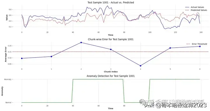
Test Sample 1001:
Chunk Errors: [0.09563164519339118, 0.11092163544298601, 0.2256666890943125, 0.16915089415034076, 0.03522613307659271, 0.1806858796623185, 0.19323275294969594]
Anomaly Flags: [0. 0. 0. 0. 0. 0. 0. 0. 0. 0. 0. 0. 0. 0. 0. 0. 0. 0. 0. 0. 0. 0. 0. 0.
 0. 0. 0. 0. 0. 0. 0. 0. 0. 0. 0. 0. 0. 0. 0. 0. 1. 1. 1. 1. 1. 1. 1. 1.
 1. 1. 1. 1. 1. 1. 1. 1. 1. 1. 1. 1. 1. 1. 1. 1. 1. 1. 1. 1. 1. 1. 1. 1.
 1. 1. 1. 1. 1. 1. 1. 1. 0. 0. 0. 0. 0. 0. 0. 0. 0. 0. 0. 0. 0. 0. 0. 0.
 0. 0. 0. 0. 1. 1. 1. 1. 1. 1. 1. 1. 1. 1. 1. 1. 1. 1. 1. 1. 1. 1. 1. 1.
 1. 1. 1. 1. 1. 1. 1. 1. 1. 1. 1. 1. 1. 1. 1. 1. 1. 1. 1. 1.]

知乎学术咨询:https://www.zhihu.com/consult/people/792359672131756032?isMe=1
担任《Mechanical System and Signal Processing》等审稿专家,擅长领域:现代信号处理,机器学习,深度学习,数字孪生,时间序列分析,设备缺陷检测、设备异常检测、设备智能故障诊断与健康管理PHM等。