数字图像处理:边缘检测
笔记来源:
1.Gradient and Laplacian Filter, Difference of Gaussians (DOG)
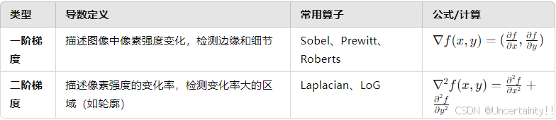
1.1 图像一阶梯度
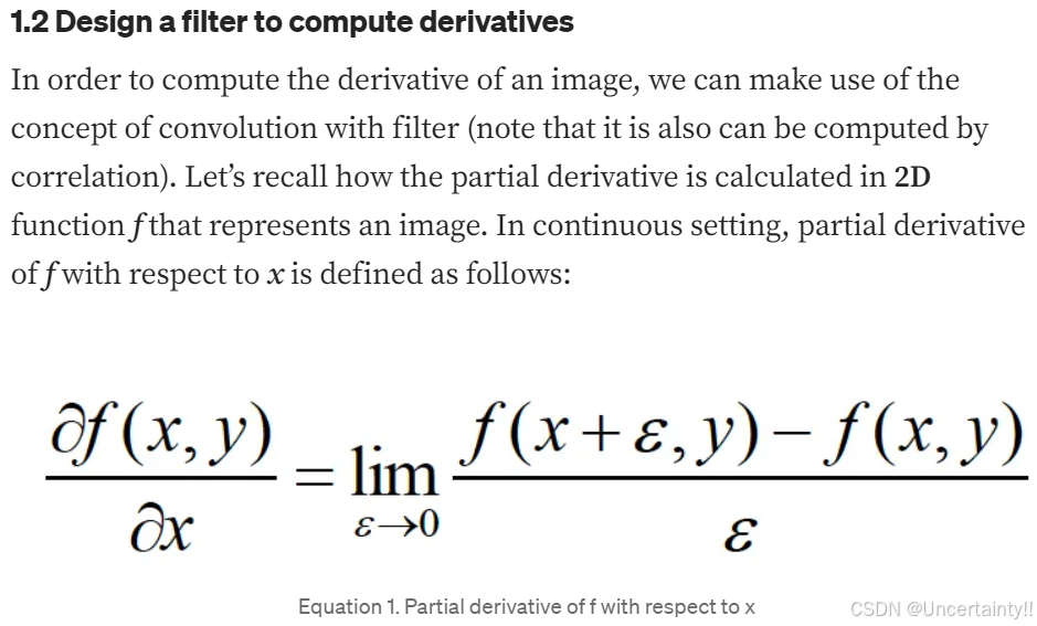


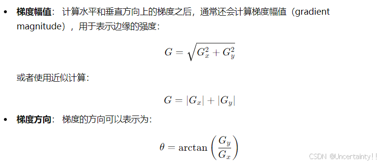
水平方向的一阶导数


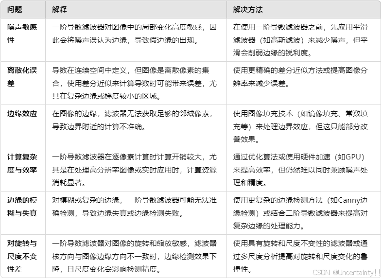
一阶导数滤波器在实际应用中难实现的原因
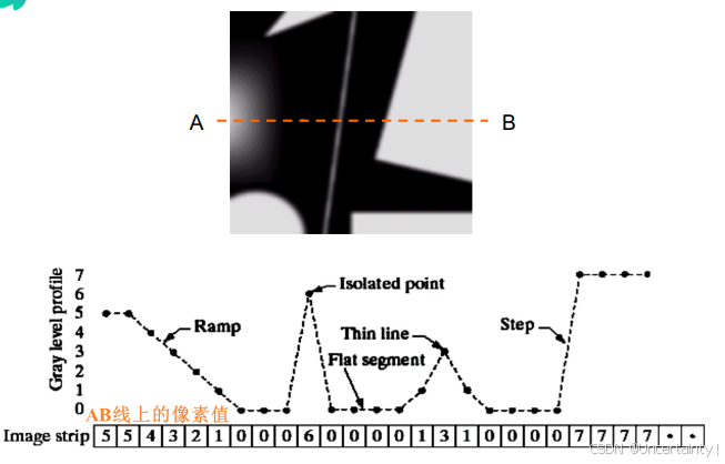
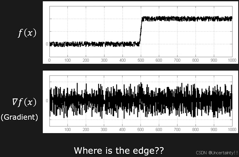
图像梯度中,一阶梯度中找局部极大值就是边缘所在处,二阶梯度中找过零点处就是边缘所在处


例如:这个函数f(x),对它求一阶导,无法找到局部极大值,即无法找到边缘
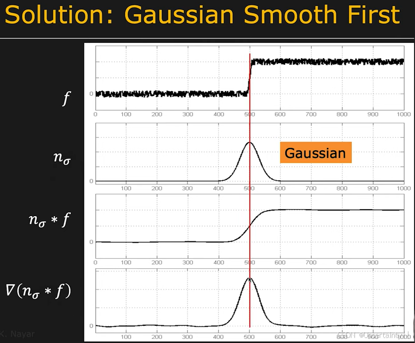
解决办法:首先对该函数进行一次高斯平滑,之后再求一阶导
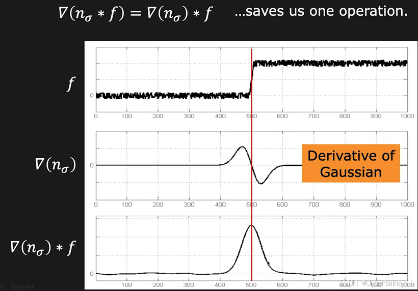
将上述操作整合一下:对f进行高斯平滑后求导 等价于 对高斯求导后与原函数卷积
1.2 Roberts算子(一阶微分算子)


1.3 Prewitt算子(一阶微分算子)


1.4 Sobel算子(一阶微分算子)


1.5 图像二阶梯度
水平方向的二阶导数


我们发现像素变化剧烈的地方(即边缘),边缘处的二阶导比一阶导更加剧烈,也就是二阶导对细节的响应更强,二阶导比一阶导更有助于图像增强
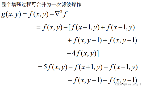
1.6 Laplace算子(二阶微分算子)


在图像上应用拉普拉斯滤波器,我们得到一个图像,突出边缘和其他不连续性

拉普拉斯滤波的结果并不是增强后的图像,我们需要从原始图像中减去拉普拉斯滤波结果,生成最终的锐化增强图像

1.7 LoG算子(Laplacian of Gaussian,二阶微分算子)
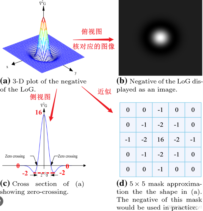
对高斯二阶导后再与原函数卷积


1.8 DoG算子(Difference of Gaussians,二阶微分算子)


1.9 代码
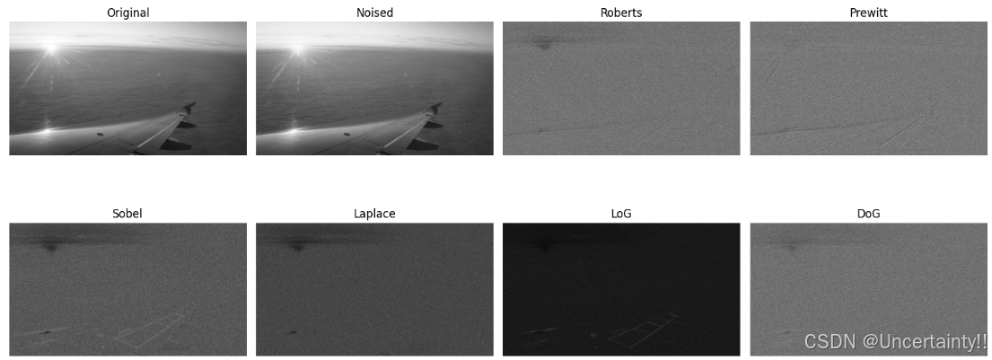
(1)选取实验用的实验图像,完成图像读取和显示,给图像加上高斯噪声;
(2)利用三种一阶微分算子(Roberts、Prewitt、Sobel)和二阶微分算子(Laplace、LoG、DoG)实现边缘检测;
python
import numpy as np
import cv2 as cv
import matplotlib.pyplot as plt

# 读取图像并转换为灰度
img_dir = r'D:\Document\Experiment\data\image1.jpg'
gray = cv.imread(img_dir, 0)

# 灰度加噪(添加高斯噪声)
mean = 0  # 均值
sigma = 20  # 标准差(调整噪声强度)
gaussian_noise = np.random.normal(mean, sigma, gray.shape)  # 生成高斯噪声
noisy_image = gray + gaussian_noise  # 将噪声加入图像
noisy_image_clipped = np.clip(noisy_image, 0, 255).astype(np.uint8)  # 剪裁到0-255范围并转换为uint8

# Roberts 算子
def roberts(image):
    kernel_x = np.array([[1, 0], [0, -1]], dtype=np.float32)
    kernel_y = np.array([[0, 1], [-1, 0]], dtype=np.float32)
    edge_x = cv.filter2D(image, -1, kernel_x)
    edge_y = cv.filter2D(image, -1, kernel_y)
    roberts_edge_image = np.sqrt(edge_x**2 + edge_y**2).astype(np.uint8)
    return roberts_edge_image

# Prewitt 算子
def prewitt(image):
    kernel_x = np.array([[1, 0, -1], [1, 0, -1], [1, 0, -1]], dtype=np.float32)
    kernel_y = np.array([[1, 1, 1], [0, 0, 0], [-1, -1, -1]], dtype=np.float32)
    edge_x = cv.filter2D(image, -1, kernel_x)
    edge_y = cv.filter2D(image, -1, kernel_y)
    prewitt_edge_image = np.sqrt(edge_x**2 + edge_y**2).astype(np.uint8)
    return prewitt_edge_image

# Sobel 算子
def sobel(image):
    edge_x = cv.Sobel(image, cv.CV_64F, 1, 0, ksize=3)
    edge_y = cv.Sobel(image, cv.CV_64F, 0, 1, ksize=3)
    sobel_edge_image = np.sqrt(edge_x**2 + edge_y**2).astype(np.uint8)
    return sobel_edge_image

# Laplace 算子
def laplace(image):
    laplace_edge_image = cv.Laplacian(image, cv.CV_64F)
    laplace_edge_image = np.uint8(np.absolute(laplace_edge_image))  # 取绝对值并转换为uint8
    return laplace_edge_image

# LoG 算子 (Laplacian of Gaussian)
def loguass(image):
    blurred = cv.GaussianBlur(image, (5, 5), 0)  # 高斯平滑
    log_edge_image = cv.Laplacian(blurred, cv.CV_64F)  # Laplace 边缘检测
    log_edge_image = np.uint8(np.absolute(log_edge_image))  # 取绝对值并转换为uint8
    return log_edge_image

# DoG 算子 (Difference of Gaussian)
def dog(image):
    blurred1 = cv.GaussianBlur(image, (5, 5), 1)  # 第一次高斯模糊
    blurred2 = cv.GaussianBlur(image, (5, 5), 2)  # 第二次高斯模糊
    dog_edge_image = blurred1 - blurred2  # 两次模糊图像的差分
    dog_edge_image = np.uint8(np.absolute(dog_edge_image))  # 取绝对值并转换为uint8
    return dog_edge_image

# 进行边缘检测
roberts_edge_image = roberts(noisy_image_clipped)
prewitt_edge_image = prewitt(noisy_image_clipped)
sobel_edge_image = sobel(noisy_image_clipped)
laplace_edge_image = laplace(noisy_image_clipped)
log_edge_image = loguass(noisy_image_clipped)
dog_edge_image = dog(noisy_image_clipped)

# 定义运算及其标题
operations = [
    ("Original", gray),  # 原始图像
    ("Noised", noisy_image_clipped),
    ("Roberts", roberts_edge_image),
    ("Prewitt", prewitt_edge_image),
    ("Sobel", sobel_edge_image),
    ("Laplace", laplace_edge_image),
    ("LoG", log_edge_image),
    ("DoG", dog_edge_image)
]

# 绘图
plt.figure(figsize=(15, 7))  # 设置绘图窗口大小
for i, (title, result) in enumerate(operations, 1):  # 遍历运算结果
    plt.subplot(2, 4, i)  # 创建子图,2行4列
    plt.title(title)  # 设置子图标题
    plt.imshow(result, cmap='gray')  # 显示图像,使用灰度颜色映射
    plt.axis('off')  # 关闭坐标轴显示

plt.tight_layout()  # 自动调整子图布局,使之不重叠
plt.show()  # 显示图像