从0开始学习机器学习--Day25--SVM作业

题目1：线性可分SVM

代码：

复制代码

import numpy as np
import scipy.io as sio
import matplotlib.pyplot as plt
from sklearn.svm import SVC

def plot_data():
    plt.scatter(X[:, 0], X[:, 1], c=y.flatten(), cmap='jet') # 输出X的维度知道其特征数，再通过y来贴标签
    plt.xlabel('x1')
    plt.ylabel('y1')


def data_boundary(model, a1, a2, b1, b2):#画决策边界
    x_min = a1 #-0.5
    x_max = a2 #4.5
    y_min = b1 #1.3
    y_max = b2 #5
    xx, yy = np.meshgrid(np.linspace(x_min, x_max, 500), np.linspace(y_min, y_max, 500))#从上述两个范围内各取500个点组成网格
    z = model.predict(np.c_[xx.flatten(), yy.flatten()])#降成一维并组成二维数组

    zz = z.reshape(xx.shape)#重塑成之前为维度，方便画图
    plt.contour(xx, yy, zz)#绘制等高线


data = sio.loadmat('./data/ex6data1.mat')
print(data.keys())
X = data['X']
y = data['y']
print(X.shape)
print(y.shape)
plot_data()
plt.show()

svc1 = SVC(C=1, kernel='linear')
svc1.fit(X, y.flatten())
y_pred1 = svc1.predict(X)
y_score1 = svc1.score(X, y.flatten())
print(y_pred1)
print(y_score1)

data_boundary(svc1, -0.5, 4.5, 1.3, 5)
plot_data()
plt.show()

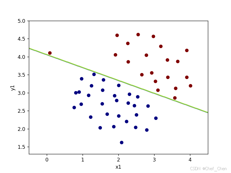
svc100 = SVC(C=100, kernel='linear')
svc100.fit(X, y.flatten())
y_pred100 = svc100.predict(X)
y_score100 = svc100.score(X, y.flatten())
print(y_pred100)
print(y_score100)

data_boundary(svc100, -0.5, 4.5, 1.3, 5)
plot_data()
plt.show()

输出：

复制代码

dict_keys(['__header__', '__version__', '__globals__', 'X', 'y'])
(51, 2)
(51, 1)
[1 1 1 1 1 1 1 1 1 1 1 1 1 1 1 1 1 1 1 1 0 0 0 0 0 0 0 0 0 0 0 0 0 0 0 0 0
 0 0 0 0 0 0 0 0 0 0 0 0 0 0]
0.9803921568627451
[1 1 1 1 1 1 1 1 1 1 1 1 1 1 1 1 1 1 1 1 0 0 0 0 0 0 0 0 0 0 0 0 0 0 0 0 0
 0 0 0 0 0 0 0 0 0 0 0 0 0 1]
1.0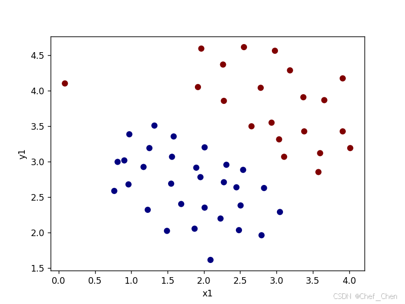

原始数据散点图

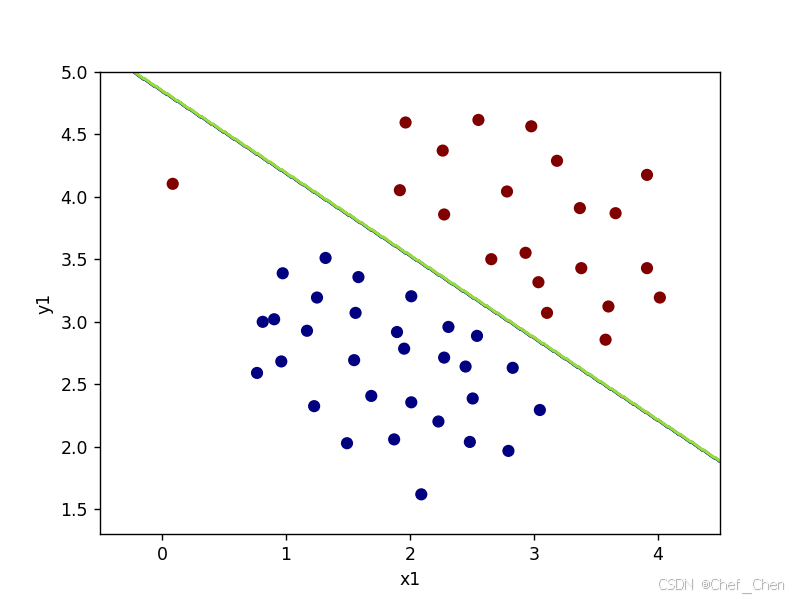
C=1时决策边界

C=1时决策边界

注意：虽然C为100时决策边界完美的把正负样本都分开来，但是此时准确度为100%，有可能左边这个点属于异常值，应该要被排除的，在实际运用中出现这种情况要警惕。

题目2：线性不可分SVM

代码：

复制代码

import numpy as np
import scipy.io as sio
import matplotlib.pyplot as plt
from sklearn.svm import SVC

def plot_data():
    plt.scatter(X[:, 0], X[:, 1], c=y.flatten(), cmap='jet') # 输出X的维度知道其特征数，再通过y来贴标签
    plt.xlabel('x1')
    plt.ylabel('y1')

def data_boundary(model, a1, a2, b1, b2):#画决策边界
    x_min = a1 #0
    x_max = a2 #1
    y_min = b1 #0.4
    y_max = b2 #1
    xx, yy = np.meshgrid(np.linspace(x_min, x_max, 500), np.linspace(y_min, y_max, 500))#从上述两个范围内各取500个点组成网格
    z = model.predict(np.c_[xx.flatten(), yy.flatten()])#降成一维并组成二维数组

    zz = z.reshape(xx.shape)#重塑成之前为维度，方便画图
    plt.contour(xx, yy, zz)#绘制等高线

data = sio.loadmat('./data/ex6data2.mat')
print(data.keys())
X = data['X']
y = data['y']
print(X.shape)
print(y.shape)
plot_data()
plt.show()

svc1 = SVC(C=1, kernel='rbf', gamma=50)
svc1.fit(X, y.flatten())
y_pred1 = svc1.predict(X)
y_score1 = svc1.score(X, y.flatten())
print(y_pred1)
print(y_score1)

data_boundary(svc1, 0, 1, 0.4, 1)
plot_data()
plt.show()

输出：

复制代码

dict_keys(['__header__', '__version__', '__globals__', 'X', 'y'])
(863, 2)
(863, 1)
[1 1 1 1 1 1 1 1 1 1 1 1 1 1 1 1 1 1 1 1 1 1 1 1 1 1 1 1 1 1 1 1 1 1 1 1 1
 1 1 1 1 1 1 1 1 1 1 1 1 1 1 1 1 1 1 1 1 1 1 1 1 1 1 1 1 1 1 1 1 1 1 1 1 1
 1 1 1 1 1 1 1 1 1 1 1 1 1 1 1 1 1 1 1 1 1 1 1 1 1 1 1 1 1 1 1 1 1 1 1 1 1
 1 1 1 1 1 1 1 1 1 1 1 1 1 1 1 1 1 1 1 1 1 1 1 1 1 1 1 1 1 1 1 1 1 1 1 1 1
 1 1 1 1 1 1 1 1 1 1 1 1 1 1 1 1 1 1 1 1 1 1 1 1 1 1 1 1 1 1 1 1 1 1 1 1 1
 1 1 1 1 1 1 1 1 0 0 0 0 0 0 0 0 0 0 0 0 0 0 0 0 0 0 0 0 0 0 0 0 0 0 0 0 0
 0 0 0 0 0 0 0 0 0 0 0 0 0 0 0 0 1 1 0 0 0 0 0 0 0 0 0 0 0 0 0 0 0 0 0 0 0
 0 0 0 0 0 0 0 0 0 0 0 0 0 0 0 0 0 0 0 0 0 0 0 0 0 0 0 0 0 0 0 0 0 0 0 0 0
 0 0 0 0 0 0 0 0 0 0 0 0 0 0 0 0 0 0 0 0 0 0 0 0 0 0 0 0 1 1 1 1 0 1 1 1 1
 1 1 1 1 1 1 1 1 1 1 1 1 1 1 1 1 1 1 1 1 1 1 1 1 1 1 1 1 1 1 1 1 1 1 1 1 1
 1 1 1 1 1 1 1 0 0 0 0 0 0 0 0 0 0 0 0 0 0 0 0 0 0 0 0 0 0 0 0 0 0 0 0 0 1
 1 1 1 1 1 1 1 1 1 1 1 1 1 1 1 1 1 1 0 0 0 1 1 1 1 1 1 1 1 1 1 1 1 1 1 1 1
 1 1 1 1 1 1 1 1 1 0 0 0 0 0 0 0 0 0 0 0 0 0 0 0 0 0 0 0 0 0 0 0 0 0 0 0 0
 0 0 0 0 0 0 0 0 0 0 0 0 0 0 0 0 0 0 0 0 0 0 0 0 0 0 0 0 0 0 0 0 0 0 0 0 1
 1 1 1 1 1 1 1 1 1 1 1 1 1 1 1 1 1 1 1 1 1 1 1 1 1 0 0 0 0 0 0 0 0 0 0 0 0
 0 0 0 0 0 0 0 0 0 0 0 0 0 0 0 0 0 0 0 0 0 1 1 1 1 1 1 1 1 1 1 1 1 1 1 1 1
 1 1 1 1 1 1 1 1 1 1 1 1 1 1 1 1 1 1 1 1 1 1 1 1 1 1 1 1 1 1 0 0 0 0 0 0 0
 0 0 0 0 0 0 0 0 0 0 0 0 0 0 0 0 0 0 0 0 0 0 0 0 0 0 0 0 0 0 0 0 0 0 0 0 0
 0 0 0 0 0 0 0 0 0 0 0 0 0 0 0 0 0 0 0 0 0 1 1 1 1 1 1 1 1 1 1 1 1 1 1 1 1
 1 1 1 1 1 1 1 1 1 1 1 1 1 1 1 1 1 1 1 1 1 1 1 1 1 1 1 1 1 1 1 1 1 1 1 1 1
 1 1 1 1 1 1 1 1 1 1 1 1 0 0 0 0 0 0 0 0 0 0 0 0 0 0 1 1 0 0 0 0 0 0 0 0 0
 0 0 0 0 0 0 0 0 0 0 0 0 0 0 0 0 0 0 0 0 0 0 0 0 0 0 0 0 0 0 0 0 0 0 0 1 1
 1 1 1 1 1 1 1 1 1 1 1 1 1 1 1 1 1 1 1 1 1 1 1 1 1 1 1 1 1 1 1 1 1 1 1 1 1
 1 1 1 1 1 1 1 1 1 1 1 1]
0.9895712630359212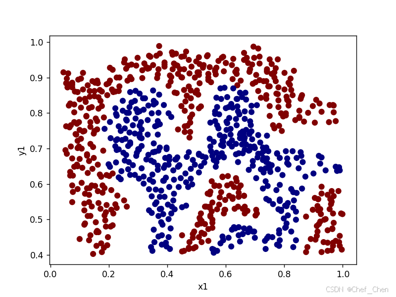

原始数据散点图

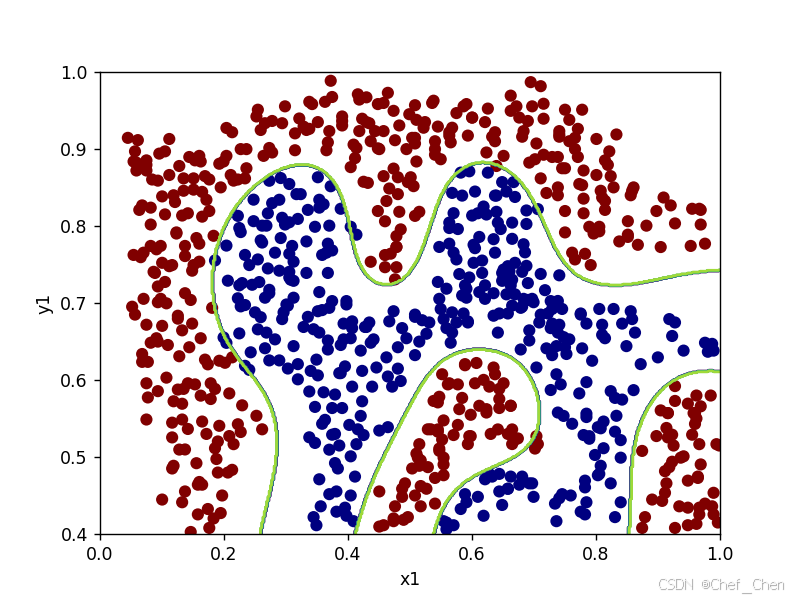
sigma=50时决策边界

题目3：寻找最优参数

代码：

复制代码

import numpy as np
import scipy.io as sio
import matplotlib.pyplot as plt
from sklearn.svm import SVC

def plot_data():
    plt.scatter(X[:, 0], X[:, 1], c=y.flatten(), cmap='jet') # 输出X的维度知道其特征数，再通过y来贴标签
    plt.xlabel('x1')
    plt.ylabel('y1')

def data_boundary(model, a1, a2, b1, b2):#画决策边界
    x_min = a1 #0
    x_max = a2 #1
    y_min = b1 #0.4
    y_max = b2 #1
    xx, yy = np.meshgrid(np.linspace(x_min, x_max, 500), np.linspace(y_min, y_max, 500))#从上述两个范围内各取500个点组成网格
    z = model.predict(np.c_[xx.flatten(), yy.flatten()])#降成一维并组成二维数组

    zz = z.reshape(xx.shape)#重塑成之前为维度，方便画图
    plt.contour(xx, yy, zz)#绘制等高线

data = sio.loadmat('./data/ex6data3.mat')
print(data.keys())
X = data['X']
y = data['y']
print(X.shape)
print(y.shape)
X_val = data['Xval']
y_val = data['yval']
plot_data()
plt.show()

C = [0.01, 0.03, 0.1, 0.3, 1, 3, 10, 30, 100]
sigmas = [0.01, 0.03, 0.1, 0.3, 1, 3, 10, 30, 100]

highest_score = 0
final_param = (0, 0)

for c in C:
    for sigma in sigmas:
        svc1 = SVC(C=c, kernel='rbf', gamma=sigma)
        svc1.fit(X, y.flatten())
        score = svc1.score(X_val, y_val.flatten())#训练好的参数在验证集预测
        if score > highest_score:
            highest_score =score
            final_param = (c, sigma)
print(highest_score, final_param)#这里的最优参数组合不唯一，任意调整上述参数可选值的顺序会使其改变，但准确度大致不变

svc2 = SVC(C=1, kernel='rbf', gamma=100)
svc2.fit(X, y.flatten())

data_boundary(svc2, -0.6, 0.4, -0.7, 0.6)
plot_data()
plt.show()

输出：

复制代码

dict_keys(['__header__', '__version__', '__globals__', 'X', 'y', 'yval', 'Xval'])
(211, 2)
(211, 1)
0.965 (0.3, 100)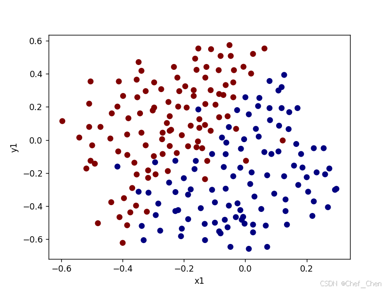

原始数据散点图

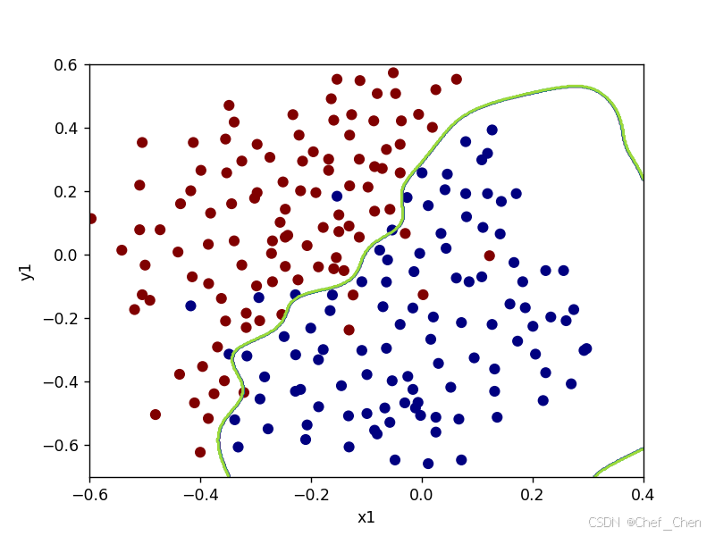
寻优后的决策边界

题目4：垃圾邮件过滤

代码：

复制代码

import scipy.io as sio
from sklearn.svm import SVC

data1 = sio.loadmat('./data/spamTrain.mat')
print(data1.keys())
X = data1['X']
y = data1['y']
print(X.shape)
print(y.shape)

data2 = sio.loadmat('./data/spamTest.mat')
print(data2.keys())
X_test = data2['Xtest']
y_test = data2['ytest']
print(X_test.shape)
print(y_test.shape)

C = [0.01, 0.03, 0.1, 0.3, 1, 3, 10, 30, 100]
# sigmas = [0.01, 0.03, 0.1, 0.3, 1, 3, 10, 30, 100]

highest_score = 0
final_param = 0

for c in C:
    svc = SVC(C=c, kernel='linear')
    svc.fit(X, y.flatten())
    score = svc.score(X_test, y_test.flatten())#训练好的参数在验证集预测
    if score > highest_score:
        highest_score = score
        final_param = c
print(highest_score, final_param)#这里的最优参数组合不唯一，任意调整上述参数可选值的顺序会使其改变，但准确度大致不变

svc1 = SVC(C=final_param, kernel='linear')
svc1.fit(X, y.flatten())
score_train = svc1.score(X, y.flatten())
score_test = svc1.score(X_test, y_test.flatten())
print(score_train)
print(score_test)

输出：

复制代码

dict_keys(['__header__', '__version__', '__globals__', 'X', 'y'])
(4000, 1899)
(4000, 1)
dict_keys(['__header__', '__version__', '__globals__', 'Xtest', 'ytest'])
(1000, 1899)
(1000, 1)
0.99 0.03
0.99425
0.99

总结：运用SVM可以帮助我们减少代码量和时间复杂度，但注意根据特征和数据集的数量选择核函数。

作业订正：https://www.bilibili.com/video/BV124411A75S?spm_id_from=333.788.videopod.episodes&vd_source=867b8ecbd62561f6cb9b4a83a368f691&p=9