- 🍨 本文为🔗365天深度学习训练营 中的学习记录博客
- 🍖 原作者:K同学啊
前言
-
LSTM 模型一直是一个很经典的模型,一般用于序列数据预测,这个可以很好的挖掘数据上下文信息,本文将使用LSTM进行糖尿病预测(二分类问题),采用LSTM+Linear解决分类问题;
-
📖 糖尿病预测之前我用随机森林做过:机器学习/数据分析案例---糖尿病预测;
-
👀 后面打算用机器学习(随机森林、SVM等)结合深度学习LSTM做一个比较完整的项目,大家可以关注一下哈;
-
LSTM讲解: 深度学习基础--LSTM学习笔记(李沐《动手学习深度学习》)
-
欢迎收藏 + 关注,本人将会持续更新
文章目录
1、数据导入和数据预处理
1、数据导入
python
import torch
import torch.nn as nn
from torch.utils.data import DataLoader, TensorDataset
import pandas as pd
import numpy as np
import matplotlib.pyplot as plt
import seaborn as sns
from sklearn.preprocessing import StandardScaler
from sklearn.model_selection import train_test_split
#设置字体
from pylab import mpl
mpl.rcParams["font.sans-serif"] = ["SimHei"]  # 显示中文
plt.rcParams['axes.unicode_minus'] = False		# 显示负号

# 数据不大,用CPU即可
device = 'cpu'

data_df = pd.read_excel('./dia.xls')

data_df.head()
| | 卡号 | 性别 | 年龄 | 高密度脂蛋白胆固醇 | 低密度脂蛋白胆固醇 | 极低密度脂蛋白胆固醇 | 甘油三酯 | 总胆固醇 | 脉搏 | 舒张压 | 高血压史 | 尿素氮 | 尿酸 | 肌酐 | 体重检查结果 | 是否糖尿病 |
| 0 | 18054421 | 0 | 38 | 1.25 | 2.99 | 1.07 | 0.64 | 5.31 | 83 | 83 | 0 | 4.99 | 243.3 | 50 | 1 | 0 |
| 1 | 18054422 | 0 | 31 | 1.15 | 1.99 | 0.84 | 0.50 | 3.98 | 85 | 63 | 0 | 4.72 | 391.0 | 47 | 1 | 0 |
| 2 | 18054423 | 0 | 27 | 1.29 | 2.21 | 0.69 | 0.60 | 4.19 | 73 | 61 | 0 | 5.87 | 325.7 | 51 | 1 | 0 |
| 3 | 18054424 | 0 | 33 | 0.93 | 2.01 | 0.66 | 0.84 | 3.60 | 83 | 60 | 0 | 2.40 | 203.2 | 40 | 2 | 0 |
| 4 | 18054425 | 0 | 36 | 1.17 | 2.83 | 0.83 | 0.73 | 4.83 | 85 | 67 | 0 | 4.09 | 236.8 | 43 | 0 | 0 |
|---|
2、数据统计
python
data_df.info()<class 'pandas.core.frame.DataFrame'>
RangeIndex: 1006 entries, 0 to 1005
Data columns (total 16 columns):
# Column Non-Null Count Dtype
--- ------ -------------- -----
0 卡号 1006 non-null int64
1 性别 1006 non-null int64
2 年龄 1006 non-null int64
3 高密度脂蛋白胆固醇 1006 non-null float64
4 低密度脂蛋白胆固醇 1006 non-null float64
5 极低密度脂蛋白胆固醇 1006 non-null float64
6 甘油三酯 1006 non-null float64
7 总胆固醇 1006 non-null float64
8 脉搏 1006 non-null int64
9 舒张压 1006 non-null int64
10 高血压史 1006 non-null int64
11 尿素氮 1006 non-null float64
12 尿酸 1006 non-null float64
13 肌酐 1006 non-null int64
14 体重检查结果 1006 non-null int64
15 是否糖尿病 1006 non-null int64
dtypes: float64(7), int64(9)
memory usage: 125.9 KB
python
data_df.describe()| | 卡号 | 性别 | 年龄 | 高密度脂蛋白胆固醇 | 低密度脂蛋白胆固醇 | 极低密度脂蛋白胆固醇 | 甘油三酯 | 总胆固醇 | 脉搏 | 舒张压 | 高血压史 | 尿素氮 | 尿酸 | 肌酐 | 体重检查结果 | 是否糖尿病 |
| count | 1.006000e+03 | 1006.000000 | 1006.000000 | 1006.000000 | 1006.000000 | 1006.000000 | 1006.000000 | 1006.000000 | 1006.000000 | 1006.000000 | 1006.000000 | 1006.000000 | 1006.000000 | 1006.000000 | 1006.000000 | 1006.000000 |
| mean | 1.838279e+07 | 0.598410 | 50.288270 | 1.152201 | 2.707475 | 0.998311 | 1.896720 | 4.857624 | 80.819085 | 76.886680 | 0.173956 | 5.562684 | 339.345427 | 64.106362 | 1.609344 | 0.444334 |
| std | 6.745088e+05 | 0.490464 | 16.921487 | 0.313426 | 0.848070 | 0.715891 | 2.421403 | 1.029973 | 12.542270 | 12.763173 | 0.379260 | 1.646342 | 84.569846 | 29.338437 | 0.772327 | 0.497139 |
| min | 1.805442e+07 | 0.000000 | 20.000000 | 0.420000 | 0.840000 | 0.140000 | 0.350000 | 2.410000 | 41.000000 | 45.000000 | 0.000000 | 2.210000 | 140.800000 | 30.000000 | 0.000000 | 0.000000 |
| 25% | 1.807007e+07 | 0.000000 | 37.250000 | 0.920000 | 2.100000 | 0.680000 | 0.880000 | 4.200000 | 72.000000 | 67.000000 | 0.000000 | 4.450000 | 280.850000 | 51.250000 | 1.000000 | 0.000000 |
| 50% | 1.807036e+07 | 1.000000 | 50.000000 | 1.120000 | 2.680000 | 0.850000 | 1.335000 | 4.785000 | 79.000000 | 76.000000 | 0.000000 | 5.340000 | 333.000000 | 62.000000 | 2.000000 | 0.000000 |
| 75% | 1.809726e+07 | 1.000000 | 60.000000 | 1.320000 | 3.220000 | 1.090000 | 2.087500 | 5.380000 | 88.000000 | 85.000000 | 0.000000 | 6.367500 | 394.000000 | 72.000000 | 2.000000 | 1.000000 |
| max | 2.026124e+07 | 1.000000 | 93.000000 | 2.500000 | 7.980000 | 11.260000 | 45.840000 | 12.610000 | 135.000000 | 119.000000 | 1.000000 | 18.640000 | 679.000000 | 799.000000 | 3.000000 | 1.000000 |
|---|
3、数据分布分析
python
# 缺失值统计
data_df.isnull().sum()卡号 0
性别 0
年龄 0
高密度脂蛋白胆固醇 0
低密度脂蛋白胆固醇 0
极低密度脂蛋白胆固醇 0
甘油三酯 0
总胆固醇 0
脉搏 0
舒张压 0
高血压史 0
尿素氮 0
尿酸 0
肌酐 0
体重检查结果 0
是否糖尿病 0
dtype: int64
python
# 数据分布、异常值分析
feature_name = {
    '性别': '性别',
    '年龄': '年龄',
    '高密度脂蛋白胆固醇': '高密度脂蛋白胆固醇',
    '低密度脂蛋白胆固醇': '低密度脂蛋白胆固醇',
    '极低密度脂蛋白胆固醇': '极低密度脂蛋白胆固醇',
    '甘油三酯': '甘油三酯',
    '总胆固醇': '总胆固醇',
    '脉搏': '脉搏',
    '舒张压': '舒张压',
    '高血压史': '高血压史',
    '尿素氮': '尿素氮',
    '肌酐': '肌酐',
    '体重检查结果': '体重检查结果',
    '是否糖尿病': '是否糖尿病'
}

# 子箱图 展示
plt.figure(figsize=(20, 20))

for i, (col, col_name) in enumerate(feature_name.items(), 1):
    plt.subplot(4, 4, i)
    # 绘制子箱图
    sns.boxplot(x=data_df["是否糖尿病"],y=data_df[col])
    # 设置标题
    plt.title(f'{col_name}的纸箱图', fontsize=10)
    plt.ylabel('数值', fontsize=12)
    plt.grid(axis='y', linestyle='--', alpha=0.7)

plt.show()
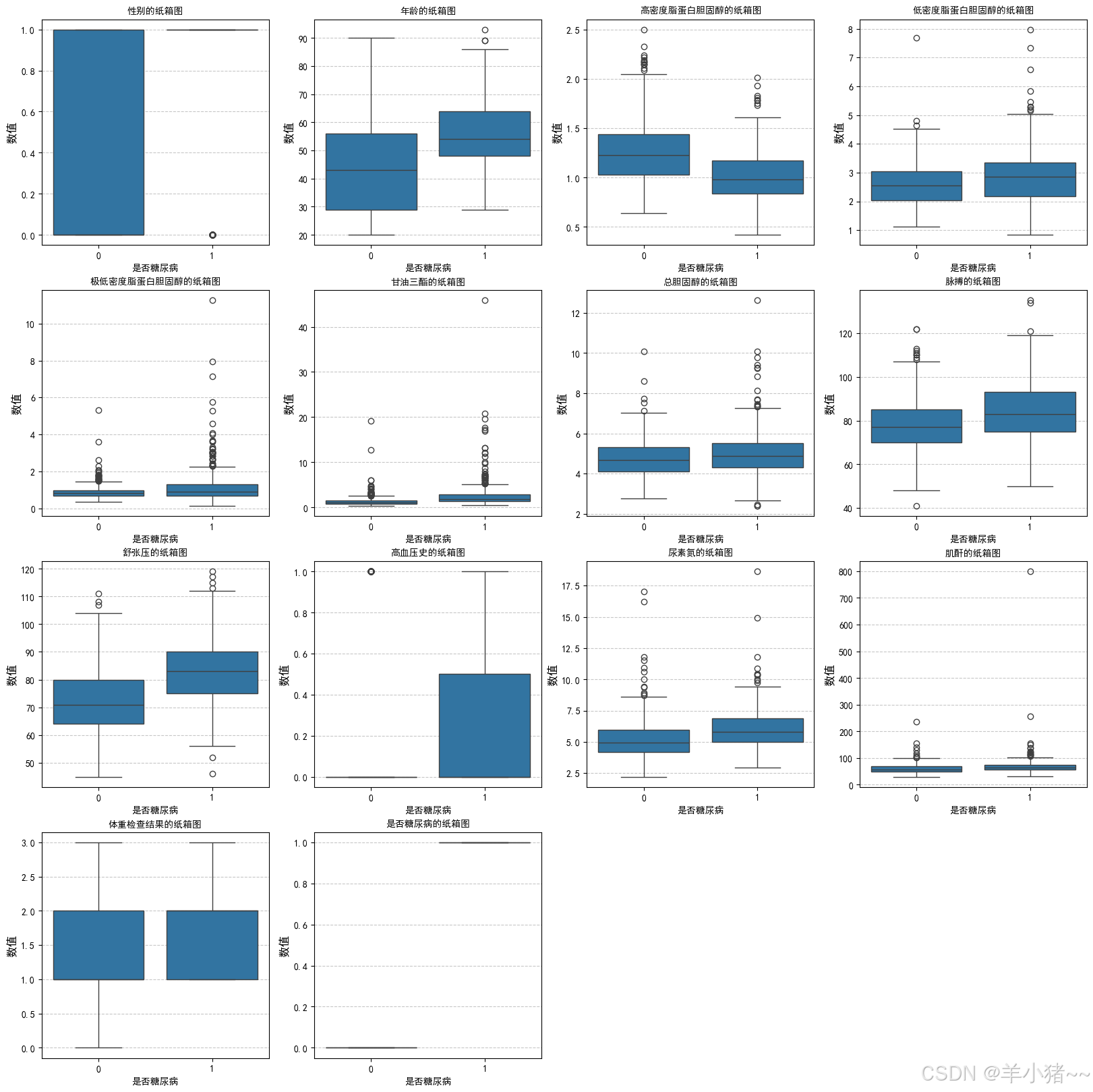
异常值分析(查阅资料后发现):
- 总数据较少;
- 特征参数受很多因素的影响,故这里假设没有异常值(数据多的时候可以进一步分析)
患糖尿病和不患糖尿病数据分布分析:
- 发现患病和不患病在:年龄、高密度蛋白固醇、低密度蛋白固醇、低密度蛋白固醇、甘油三肪、舒张压、高血压、尿素的相关因素等数据因素有关
4、相关性分析
python
plt.figure(figsize=(15, 10))
sns.heatmap(data_df.corr(), annot=True, fmt=".2f")
plt.show()
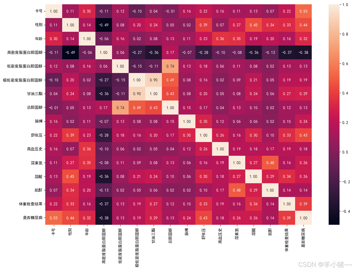
高密度蛋白胆固醇存在负相关,故删除该特征
2、数据标准化和划分
时间步长为1
python
# 特征选择
x = data_df.drop(['卡号', '高密度脂蛋白胆固醇', '是否糖尿病'], axis=1)
y = data_df['是否糖尿病']

# 数据标准化(数据之间差别大), 二分类问题,y不需要做标准化
sc = StandardScaler()
x = sc.fit_transform(x)

# 转换为tensors数据
x = torch.tensor(np.array(x), dtype=torch.float32)
y = torch.tensor(np.array(y), dtype=torch.int64)

# 数据划分, 训练:测试 = 8: 2
x_train, x_test, y_train, y_test = train_test_split(x, y, test_size=0.2 ,random_state=42)

# 维度设置, [batch_size, seq, features], 当然不设置也没事,因为这样默认** 设置 seq 为 1**
x_train = x_train.unsqueeze(1)
x_test = x_test.unsqueeze(1)

# 查看维度
x_train.shape, y_train.shape(torch.Size([804, 1, 13]), torch.Size([804]))
python
# 构建数据集
batch_size = 16

train_dl = DataLoader(TensorDataset(x_train, y_train),
                      batch_size=batch_size,
                      shuffle=True
                      )

test_dl = DataLoader(TensorDataset(x_test, y_test),
                     batch_size=batch_size,
                     shuffle=False
                     )
python
for X, Y in train_dl:
    print(X.shape)
    print(Y.shape)
break torch.Size([16, 1, 13])
torch.Size([16])3、创建模型
python
class Model_lstm(nn.Module):
    def __init__(self):
        super().__init__()

        '''
        模型结构:
            1、两层lstm
            2、一层linear
        '''

        self.lstm1 = nn.LSTM(input_size=13, hidden_size=200,
                             num_layers=1, batch_first=True)
        self.lstm2 = nn.LSTM(input_size=200, hidden_size=200,
                             num_layers=1, batch_first=True)
        # 展开,分类
        self.lc1 = nn.Linear(200, 2)

    def forward(self, x):
        out, hidden1 = self.lstm1(x)
        out, _ = self.lstm2(out, hidden1)  # 将上一个层的最后隐藏层状态,作为lstm2的这一层的隐藏层状态
        out = self.lc1(out)
        return out

model = Model_lstm().to(device)

modelModel_lstm(
(lstm1): LSTM(13, 200, batch_first=True)
(lstm2): LSTM(200, 200, batch_first=True)
(lc1): Linear(in_features=200, out_features=2, bias=True)
)
python
model(torch.randn(8, 1, 13)).shapetorch.Size([8, 1, 2])4、模型训练
1、创建训练集
python
def train(dataloader, model, loss_fn, opt):
    size = len(dataloader.dataset)
    num_batch = len(dataloader)

    train_acc, train_loss = 0.0, 0.0

    for X, y in dataloader:
        X, y = X.to(device), y.to(device)

        pred = model(X).view(-1, 2)
        loss = loss_fn(pred, y)

        # 梯度设置
        opt.zero_grad()
        loss.backward()
        opt.step()

        train_loss += loss.item()
        # 求最大概率配对
        train_acc += (pred.argmax(1) == y).type(torch.float).sum().item()

    train_acc /= size
    train_loss /= num_batch

    return train_acc, train_loss
2、创建测试集函数
python
def test(dataloader, model, loss_fn):
    size = len(dataloader.dataset)
    num_batch = len(dataloader)

    test_acc, test_loss = 0.0, 0.0

    with torch.no_grad():
        for X, y in dataloader:
            X, y = X.to(device), y.to(device)

            pred = model(X).view(-1, 2)
            loss = loss_fn(pred, y)

            test_loss += loss.item()
            # 求最大概率配对
            test_acc += (pred.argmax(1) == y).type(torch.float).sum().item()

    test_acc /= size
    test_loss /= num_batch

    return test_acc, test_loss
3、设置超参数
python
learn_rate = 1e-4
opt = torch.optim.Adam(model.parameters(), lr=learn_rate)
loss_fn = nn.CrossEntropyLoss()
5、模型训练
python
epochs = 50

train_acc, train_loss, test_acc, test_loss = [], [], [], []

for i in range(epochs):
    model.train()
    epoch_train_acc, epoch_train_loss = train(train_dl, model, loss_fn, opt)

    model.eval()
    epoch_test_acc, epoch_test_loss = test(test_dl, model, loss_fn)

    train_acc.append(epoch_train_acc)
    train_loss.append(epoch_train_loss)
    test_acc.append(epoch_test_acc)
    test_loss.append(epoch_test_loss)

    # 输出
    template = ('Epoch:{:2d}, Train_acc:{:.1f}%, Train_loss:{:.3f}, Test_acc:{:.1f}%, Test_loss:{:.3f}')
    print(template.format(i + 1, epoch_train_acc*100, epoch_train_loss, epoch_test_acc*100, epoch_test_loss))

print("---------------Done---------------")Epoch: 1, Train_acc:58.5%, Train_loss:0.677, Test_acc:75.7%, Test_loss:0.655
Epoch: 2, Train_acc:71.0%, Train_loss:0.643, Test_acc:77.2%, Test_loss:0.606
Epoch: 3, Train_acc:75.2%, Train_loss:0.590, Test_acc:79.7%, Test_loss:0.533
Epoch: 4, Train_acc:76.9%, Train_loss:0.524, Test_acc:80.2%, Test_loss:0.469
Epoch: 5, Train_acc:77.5%, Train_loss:0.481, Test_acc:79.7%, Test_loss:0.436
Epoch: 6, Train_acc:78.4%, Train_loss:0.470, Test_acc:79.7%, Test_loss:0.419
Epoch: 7, Train_acc:78.6%, Train_loss:0.452, Test_acc:80.7%, Test_loss:0.412
Epoch: 8, Train_acc:78.5%, Train_loss:0.449, Test_acc:80.7%, Test_loss:0.406
Epoch: 9, Train_acc:78.7%, Train_loss:0.444, Test_acc:80.7%, Test_loss:0.400
Epoch:10, Train_acc:79.0%, Train_loss:0.435, Test_acc:81.2%, Test_loss:0.395
Epoch:11, Train_acc:78.4%, Train_loss:0.428, Test_acc:81.2%, Test_loss:0.391
Epoch:12, Train_acc:79.1%, Train_loss:0.428, Test_acc:81.2%, Test_loss:0.388
Epoch:13, Train_acc:79.0%, Train_loss:0.421, Test_acc:80.7%, Test_loss:0.385
Epoch:14, Train_acc:79.2%, Train_loss:0.415, Test_acc:81.7%, Test_loss:0.382
Epoch:15, Train_acc:79.1%, Train_loss:0.415, Test_acc:81.7%, Test_loss:0.379
Epoch:16, Train_acc:79.7%, Train_loss:0.422, Test_acc:81.7%, Test_loss:0.377
Epoch:17, Train_acc:79.5%, Train_loss:0.410, Test_acc:81.7%, Test_loss:0.375
Epoch:18, Train_acc:79.2%, Train_loss:0.406, Test_acc:81.7%, Test_loss:0.374
Epoch:19, Train_acc:80.3%, Train_loss:0.407, Test_acc:82.2%, Test_loss:0.372
Epoch:20, Train_acc:80.1%, Train_loss:0.409, Test_acc:81.2%, Test_loss:0.370
Epoch:21, Train_acc:80.2%, Train_loss:0.397, Test_acc:80.7%, Test_loss:0.368
Epoch:22, Train_acc:81.0%, Train_loss:0.399, Test_acc:81.7%, Test_loss:0.367
Epoch:23, Train_acc:80.7%, Train_loss:0.396, Test_acc:81.2%, Test_loss:0.365
Epoch:24, Train_acc:81.0%, Train_loss:0.401, Test_acc:81.7%, Test_loss:0.363
Epoch:25, Train_acc:81.1%, Train_loss:0.392, Test_acc:82.2%, Test_loss:0.363
Epoch:26, Train_acc:81.2%, Train_loss:0.385, Test_acc:82.2%, Test_loss:0.362
Epoch:27, Train_acc:80.6%, Train_loss:0.392, Test_acc:82.2%, Test_loss:0.361
Epoch:28, Train_acc:80.5%, Train_loss:0.382, Test_acc:81.2%, Test_loss:0.358
Epoch:29, Train_acc:81.1%, Train_loss:0.386, Test_acc:81.7%, Test_loss:0.358
Epoch:30, Train_acc:80.7%, Train_loss:0.380, Test_acc:82.2%, Test_loss:0.358
Epoch:31, Train_acc:81.5%, Train_loss:0.378, Test_acc:81.7%, Test_loss:0.357
Epoch:32, Train_acc:80.6%, Train_loss:0.373, Test_acc:81.2%, Test_loss:0.356
Epoch:33, Train_acc:81.3%, Train_loss:0.373, Test_acc:81.7%, Test_loss:0.357
Epoch:34, Train_acc:80.8%, Train_loss:0.378, Test_acc:81.7%, Test_loss:0.354
Epoch:35, Train_acc:81.5%, Train_loss:0.372, Test_acc:81.2%, Test_loss:0.355
Epoch:36, Train_acc:81.5%, Train_loss:0.368, Test_acc:81.2%, Test_loss:0.354
Epoch:37, Train_acc:81.2%, Train_loss:0.368, Test_acc:80.7%, Test_loss:0.354
Epoch:38, Train_acc:81.2%, Train_loss:0.369, Test_acc:81.2%, Test_loss:0.353
Epoch:39, Train_acc:81.7%, Train_loss:0.365, Test_acc:81.2%, Test_loss:0.354
Epoch:40, Train_acc:81.5%, Train_loss:0.363, Test_acc:81.2%, Test_loss:0.355
Epoch:41, Train_acc:81.7%, Train_loss:0.358, Test_acc:81.2%, Test_loss:0.354
Epoch:42, Train_acc:81.7%, Train_loss:0.355, Test_acc:81.2%, Test_loss:0.353
Epoch:43, Train_acc:81.3%, Train_loss:0.353, Test_acc:80.7%, Test_loss:0.354
Epoch:44, Train_acc:82.0%, Train_loss:0.355, Test_acc:80.7%, Test_loss:0.354
Epoch:45, Train_acc:81.7%, Train_loss:0.353, Test_acc:79.7%, Test_loss:0.354
Epoch:46, Train_acc:82.1%, Train_loss:0.354, Test_acc:80.2%, Test_loss:0.354
Epoch:47, Train_acc:82.0%, Train_loss:0.349, Test_acc:80.2%, Test_loss:0.356
Epoch:48, Train_acc:82.1%, Train_loss:0.350, Test_acc:80.2%, Test_loss:0.356
Epoch:49, Train_acc:82.0%, Train_loss:0.345, Test_acc:80.7%, Test_loss:0.355
Epoch:50, Train_acc:81.8%, Train_loss:0.344, Test_acc:80.7%, Test_loss:0.355
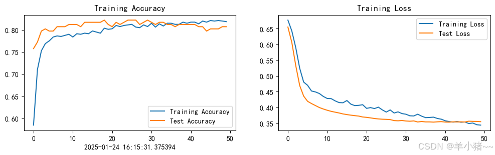
---------------Done---------------6、模型结果展示
python
from datetime import datetime
current_time = datetime.now()

epochs_range = range(epochs)

plt.figure(figsize=(12, 3))
plt.subplot(1, 2, 1)

plt.plot(epochs_range, train_acc, label='Training Accuracy')
plt.plot(epochs_range, test_acc, label='Test Accuracy')
plt.legend(loc='lower right')
plt.title('Training Accuracy')
plt.xlabel(current_time)

plt.subplot(1, 2, 2)
plt.plot(epochs_range, train_loss, label='Training Loss')
plt.plot(epochs_range, test_loss, label='Test Loss')
plt.legend(loc='upper right')
plt.title('Training Loss')
plt.show()
7、预测
python
test_x = x_test[0].reshape(1, 1, 13)

pred = model(test_x.to(device)).reshape(-1, 2)
res = pred.argmax(1).item()

print(f"预测结果: {res}, (1: 患病; 0: 不患病)")预测结果: 1, (1: 患病; 0: 不患病)