三 模型创建与nn.Module
3.1 nn.Module
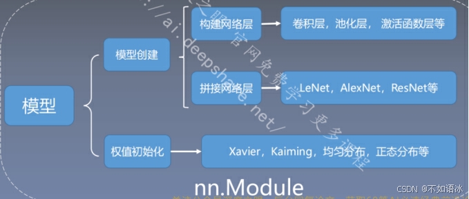
模型构建两要素:
- 构建子模块------init()
- 拼接子模块------forward()

一个module可以有多个module;
一个module相当于一个运算,都必须实现forward函数;
每一个module有8个字典管理属性。
self._parameters = OrderedDict()
self._buffers = OrderedDict()
self._backward_hooks = OrderedDict()
self._forward_hooks = OrderedDict()
self._forward_pre_hooks = OrderedDict()
self._state_dict_hooks = OrderedDict()
self._load_state_dict_pre_hooks = OrderedDict()
self._modules = OrderedDict()
3.2 网络容器
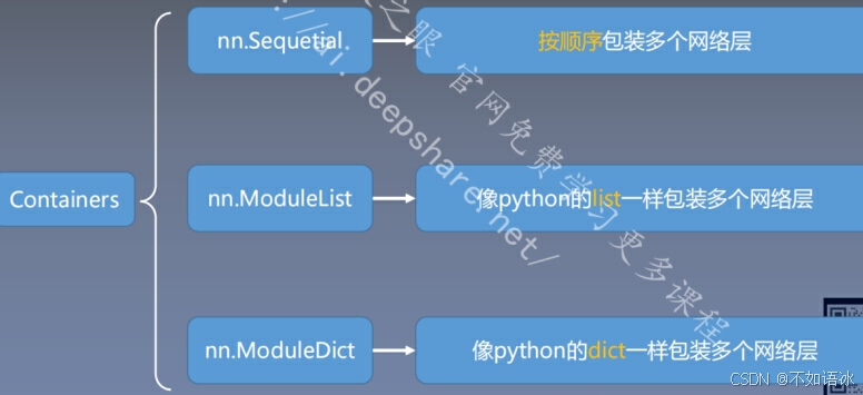
nn.Sequential()
是nn.Module()的一个容器,用于按照顺序包装一组网络层;
顺序性:网络层之间严格按照顺序构建;
自带forward():
各网络层之间严格按顺序执行,常用于block构建
class LeNetSequential(nn.Module):
def init(self, classes):
super(LeNetSequential, self).init()
self.features = nn.Sequential(
nn.Conv2d(3, 6, 5),
nn.ReLU(),
nn.MaxPool2d(kernel_size=2, stride=2),
nn.Conv2d(6, 16, 5),
nn.ReLU(),
nn.MaxPool2d(kernel_size=2, stride=2),)
self.classifier = nn.Sequential(
nn.Linear(16*5*5, 120),
nn.ReLU(),
nn.Linear(120, 84),
nn.ReLU(),
nn.Linear(84, classes),)
def forward(self, x):
x = self.features(x)
x = x.view(x.size()0, -1)
x = self.classifier(x)
return x
nn.ModuleList()
是nn.Module的容器,用于包装网络层,以迭代方式调用网络层。
主要方法:
append():在ModuleList后面添加网络层;
extend():拼接两个ModuleList.
Insert():指定在ModuleList中插入网络层。
nn.ModuleList:迭代性,常用于大量重复网 构建,通过for循环实现重复构建
class ModuleList(nn.Module):
def init(self):
super(ModuleList, self).init()
self.linears = nn.ModuleList(nn.Linear(10, 10) for i in range(20))
def forward(self, x):
for i, linear in enumerate(self.linears):
x = linear(x)
return x
nn.ModuleDict()
以索引方式调用网络层
主要方法:
• clear():清空ModuleDict
• items():返回可迭代的键值对(key-value pairs)
• keys():返回字典的键(key)
• values():返回字典的值(value)
• pop():返回一对键值,并从字典中删除
n.ModuleDict:索引性,常用于可选择的网络层
class ModuleDict(nn.Module):
def init(self):
super(ModuleDict, self).init()
self.choices = nn.ModuleDict({
'conv': nn.Conv2d(10, 10, 3),
'pool': nn.MaxPool2d(3)
})
self.activations = nn.ModuleDict({
'relu': nn.ReLU(),
'prelu': nn.PReLU()
})
def forward(self, x, choice, act):
x = self.choiceschoice(x)
x = self.activationsact(x)
return x
3.3卷积层
nn.ConV2d()
nn.Conv2d(in_channels, out_channels,kernel_size, stride=1,padding=0, dilation=1, groups=1, bias=True, padding_mode='zeros')
in_channels:输入通道数,比如RGB图像是3,而后续的网络层的输入通道数为前一卷积层的输出通道数;
out_channels:输出通道数,等价于卷积核个数
kernel_size:卷积核尺寸
stride:步
padding:填充个数
dilation:空洞卷积大小
groups:分组卷积设置
bias:偏置
conv_layer = nn.Conv2d(3, 1, 3) # input:(i, o, size) weights:(o, i , h, w)
nn.init.xavier_normal_(conv_layer.weight.data)
calculation
img_conv = conv_layer(img_tensor)
这里使用 input*channel 为 3,output_channel 为 1 ,卷积核大小为 3×3 的卷积核nn.Conv2d(3, 1, 3),使用nn.init.xavier_normal*()方法初始化网络的权值。
我们通过`conv_layer.weight.shape`查看卷积核的 shape 是`(1, 3, 3, 3)`,对应是`(output_channel, input_channel, kernel_size, kernel_size)`。所以第一个维度对应的是卷积核的个数,每个卷积核都是`(3,3,3)`。虽然每个卷积核都是 3 维的,执行的却是 2 维卷积。
转置卷积nn.ConvTranspose2d
转置卷积又称为反卷积(Deconvolution)和部分跨越卷积(Fractionally-stridedConvolution) ,用于对图像进行上采样(UpSample)
为什么称为转置卷积?
假设图像尺寸为4*4,卷积核为3*3,padding=0,stride=1
正常卷积:

转置卷积:
假设图像尺寸为2*2,卷积核为3*3,padding=0,stride=1

nn.ConvTranspose2d(in_channels, out_channels,
kernel_size,
stride=1,
padding=0,
output_padding=0,
groups=1,
bias=True,
dilation=1, padding_mode='zeros')
输出尺寸计算:


flag = 1
flag = 0
if flag:
conv_layer = nn.ConvTranspose2d(3, 1, 3, stride=2) # input:(i, o, size)
nn.init.xavier_normal_(conv_layer.weight.data)
calculation
img_conv = conv_layer(img_tensor)
print("卷积前尺寸:{}\n卷积后尺寸:{}".format(img_tensor.shape, img_conv.shape))
img_conv = transform_invert(img_conv0, 0:1, ..., img_transform)
img_raw = transform_invert(img_tensor.squeeze(), img_transform)
plt.subplot(122).imshow(img_conv, cmap='gray')
plt.subplot(121).imshow(img_raw)
plt.show()
3.4池化层nn.MaxPool2d && nn.AvgPool2d
池化运算:对信号进行 "收集"并 "总结",类似水池收集水资源,因而
得名池化层
"收集":多变少
"总结":最大值/平均值
nn.MaxPool2d
nn.MaxPool2d(kernel_size, stride=None,
padding=0, dilation=1,
return_indices=False,
ceil_mode=False)
主要参数:
• kernel_size:池化核尺寸
• stride:步长
• padding :填充个数
• dilation:池化核间隔大小
• ceil_mode:尺寸向上取整
• return_indices:记录池化像素索引
flag = 1
flag = 0
if flag:
maxpool_layer = nn.MaxPool2d((2, 2), stride=(2, 2)) # input:(i, o, size) weights:(o, i , h, w)
img_pool = maxpool_layer(img_tensor)
nn.AvgPool2d
nn.AvgPool2d(kernel_size,
stride=None,
padding=0,
ceil_mode=False,
count_include_pad=True,
divisor_override=None)
主要参数:
• kernel_size:池化核尺寸
• stride:步长
• padding :填充个数
• ceil_mode:尺寸向上取整
• count_include_pad:填充值用于计算
• divisor_override :除法因子
avgpoollayer = nn.AvgPool2d((2, 2), stride=(2, 2)) # input:(i, o, size) weights:(o, i , h, w)
img_pool = avgpoollayer(img_tensor)
img_tensor = torch.ones((1, 1, 4, 4))
avgpool_layer = nn.AvgPool2d((2, 2), stride=(2, 2), divisor_override=3)
img_pool = avgpool_layer(img_tensor)
print("raw_img:\n{}\npooling_img:\n{}".format(img_tensor, img_pool))
nn.MaxUnpool2d
功能:对二维信号(图像)进行最大值池化
上采样
主要参数:
• kernel_size:池化核尺寸
• stride:步长
• padding :填充个数
pooling
img_tensor = torch.randint(high=5, size=(1, 1, 4, 4), dtype=torch.float)
maxpool_layer = nn.MaxPool2d((2, 2), stride=(2, 2), return_indices=True)
img_pool, indices = maxpool_layer(img_tensor)
unpooling
img_reconstruct = torch.randn_like(img_pool, dtype=torch.float)
maxunpool_layer = nn.MaxUnpool2d((2, 2), stride=(2, 2))
img_unpool = maxunpool_layer(img_reconstruct, indices)
print("raw_img:\n{}\nimg_pool:\n{}".format(img_tensor, img_pool))
print("img_reconstruct:\n{}\nimg_unpool:\n{}".format(img_reconstruct, img_unpool))
3.5线性层
nn.Linear(in_features, out_features, bias=True)
功能:对一维信号(向量)进行线性组合
主要参数:
• in_features:输入结点数
• out_features:输出结点数
• bias :是否需要偏置
计算公式:y = 𝒙𝑾𝑻 + 𝒃𝒊𝒂s
inputs = torch.tensor(\[1., 2, 3])
linear_layer = nn.Linear(3, 4)
linear_layer.weight.data = torch.tensor(\[1., 1., 1.,
2., 2., 2.,
3., 3., 3.,
4., 4., 4.])
linear_layer.bias.data.fill_(0.5)
output = linear_layer(inputs)
print(inputs, inputs.shape)
print(linear_layer.weight.data, linear_layer.weight.data.shape)
print(output, output.shape)
3.6 激活函数层
nn.Sigmoid
nn.tanh:
nn.ReLU
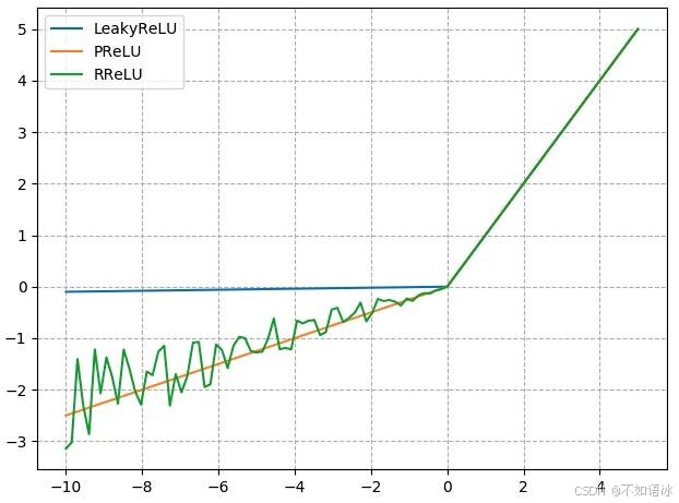
nn.LeakyReLU
negative_slope: 负半轴斜率
nn.PReLU
init: 可学习斜率
nn.RReLU
lower: 均匀分布下限
upper:均匀分布上限
参考资料
深度之眼课程