HGCN论文阅读 - 技术栈

HGCN结构

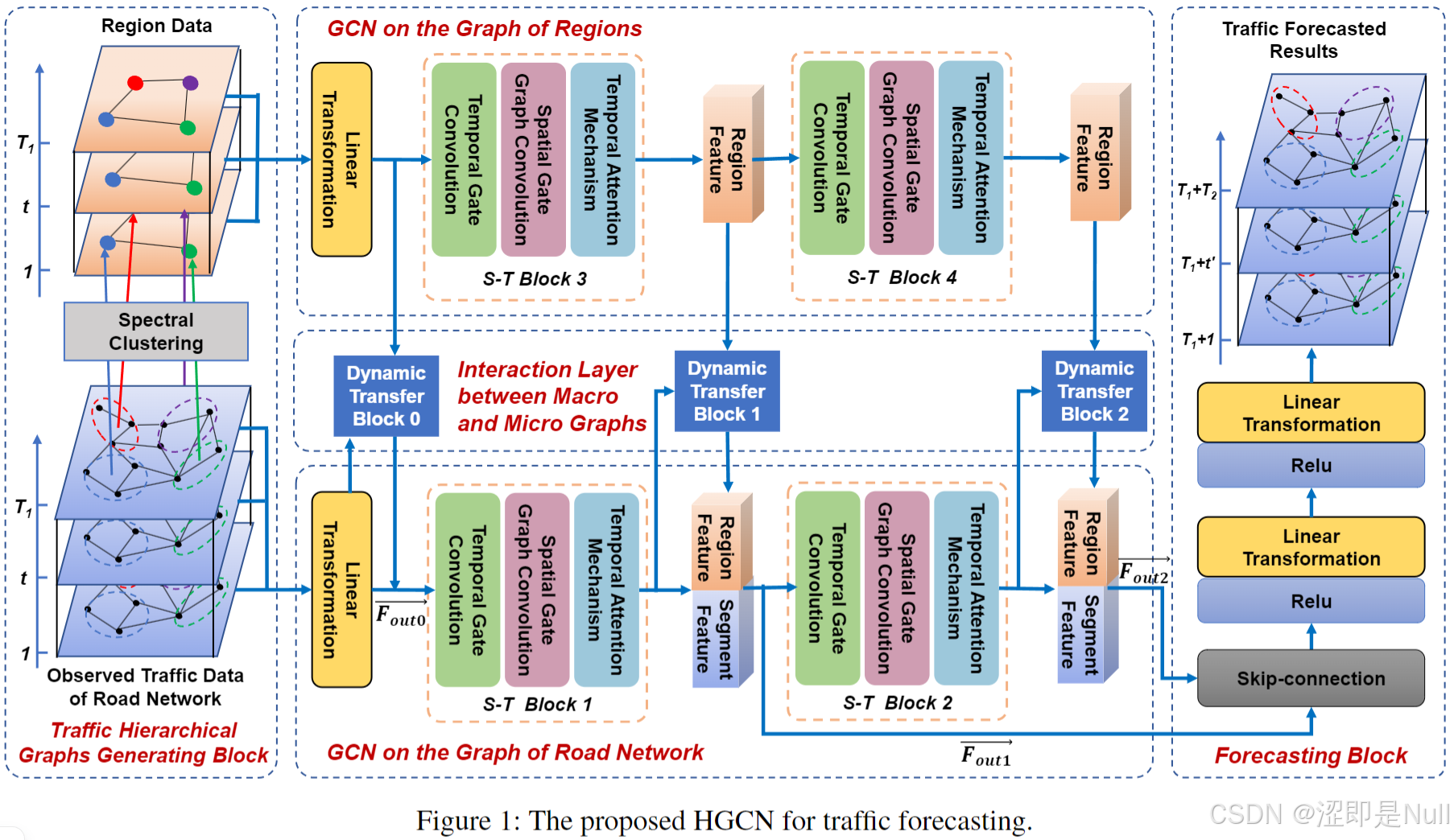
本篇论文解决交通预测问题共分为五个部分，分别是谱聚类（Spectral Clustering）、区域图山的GCN（GCN on the Graph of Regions）、道路网络图山的GCN（GCN on the Graph of Road Network）、宏观图和微观图之间的交互层（Interaction Layer between Macro and Micro Graphs）、交通预测块（Traffic Forecasting Block）。

1 生成交通层次图（Spectral Clustering）

1.1 构建微观道路网络图

所谓 "微观" ，就是道路图上节点的交通数据（如速度、流量或密度）。

1.2 构建宏观区域图

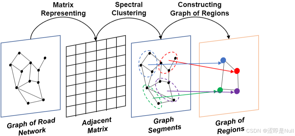
所谓 "宏观区域" ，就是指把之前的微观节点聚类为一个区域。本文采用谱聚类方法，对道路网络图进行处理，从而构建区域的宏观图。如上图所示，一共分为4步：

获取邻接矩阵：首先从道路网络图中获得邻接矩阵。
谱聚类：对邻接矩阵的拉普拉斯矩阵进行谱聚类，将整个道路网络划分为若干簇。每个簇即视作区域图中的一个宏观节点。
区域特征计算：每个宏观节点（4个小点儿）的特征由该簇内所有微观节点特征的均值和最小值组合而成。
构造宏观图边：基于微观图构造宏观图。

2 区域图上的GCN（GCN on the Graph of Regions）

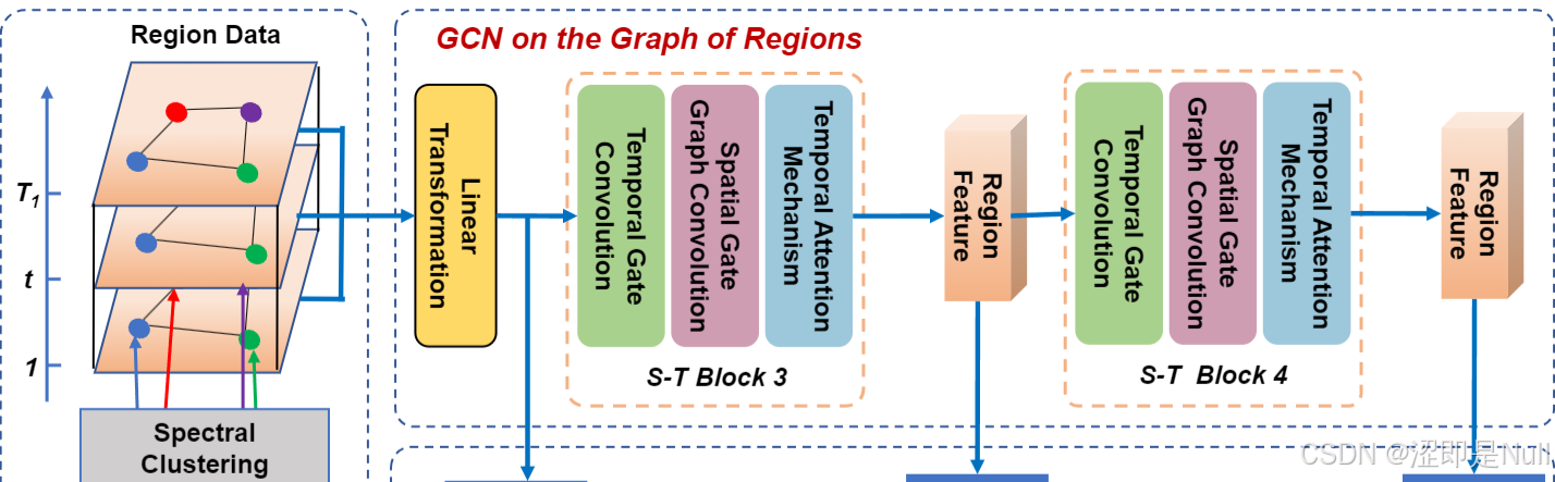
针对第一步中产生的基于区域的宏观图（Region Data），先来一个线性变换（Linear Transformation）对其进行初步转换。其主要目的是将输入数据投影到一个新的特征空间，以便后续的图卷积操作能够更有效地学习数据表示。

python 复制代码

# 线性变换：将 in_dim(1) 维度转换为 residual_channels(32) 维度
self.start_conv_cluster = nn.Conv2d(in_channels=in_dim_cluster,
                                    out_channels=residual_channels,
                                    kernel_size=(1, 1))

input_c = input_cluster
x_cluster = self.bn_cluster(input_c)
x_cluster = self.start_conv_cluster(x_cluster)  # 关于区域图的特征张量

接下来，是连续的两次时空图卷积（S-T Block）。在第一个时空卷积块（S-T Block）中，采用一个较小的卷积核，感受野增长很慢，模型主要处理一些最近的数据。比如：突发事件、红绿灯导致的交通波动、局部区域的流量变化。

在第二个时空卷积块中，它的输入已经包含了过去几个时间步的汇总信息，因此可以处理处理更长时间范围的数据。比如：上下班高峰、天气影响、节假日模式。

python 复制代码

# 计算区域图的邻接矩阵 new_supports_cluster 
A_cluster = F.relu(torch.mm(self.nodevec1_c, self.nodevec2_c))
d_c = 1 / (torch.sum(A_cluster, -1))
D_c = torch.diag_embed(d_c)
A_cluster = torch.matmul(D_c, A_cluster)
new_supports_cluster = self.supports_cluster + [A_cluster]

# 定义卷积块
self.block_cluster1 = GCNPool(dilation_channels, dilation_channels, cluster_nodes, length - 6, 3, dropout,
                              cluster_nodes,
                              self.supports_len)

# 卷积
x_cluster = self.block_cluster1(x_cluster, new_supports_cluster)

3 道路网络图上的 GCN（GCN on the Graph of Road Network）

道路网络图上的 GCN 和区域图上的 GCN 算法基本相同，只不过输入数据从区域图变成了道路节点图，也就是最传统的卷积方式。

4 宏观图和微观图之间的交互层（Interaction Layer between Macro and Micro Graphs）

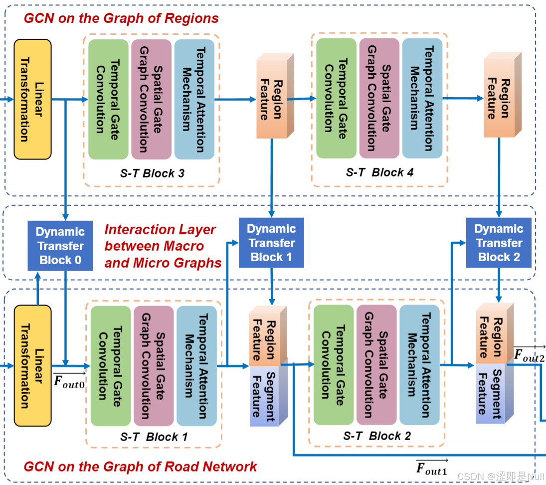
如上图所示，在区域图和道路网之间存在一个动态传递模块（Dynamic Transfer Block），用于融合区域特征与道路段特征。

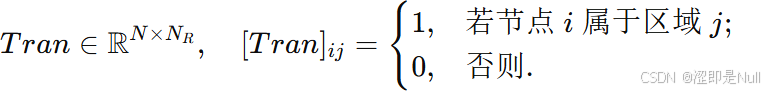
首先，构造一个传递函数 Tran 。对于道路节点 i 与区域 j 的对应关系，如果节点 i 属于区域 j，则将区域 j 的特征复制并与道路段 i 的特征级联。

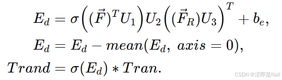
因为交通数据具有动态变化的特性，道路段与区域之间的关系也应随之变化。因此作者采用了注意力机制优化传递函数。其中为注意力分数，减去均值有助于消除不同特征维度间数值分布的偏差，使后续计算更稳定。

python 复制代码

# 道路网络特征
c1 = seq  
f1 = self.conv1(c1).squeeze(1)#b,n,l

# 区域特征
c2 = seq_cluster.permute(0,3,1,2)#b,c,n,l->b,l,n,c
f2 = self.conv2(c2).squeeze(1)#b,c,n

logits=torch.sigmoid(torch.matmul(torch.matmul(f1,self.w),f2)+self.b)
a = torch.mean(logits, 1, True)
logits = logits - a
logits = torch.sigmoid(logits)

coefs = (logits)*self.transmit

最后，按照上述方法进行特征传递。设道路特征为，区域特征为。

python 复制代码

x = self.start_conv(x)  # 道路网特征张量
x_cluster = self.start_conv_cluster(x_cluster)  # 区域图特征张量
transmit1 = self.transmit1(x, x_cluster)
x_1 = (torch.einsum('bmn,bcnl->bcml', transmit1, x_cluster))
x = self.gate1(x, x_1)

5 交通预测块（Traffic Forecasting Block）

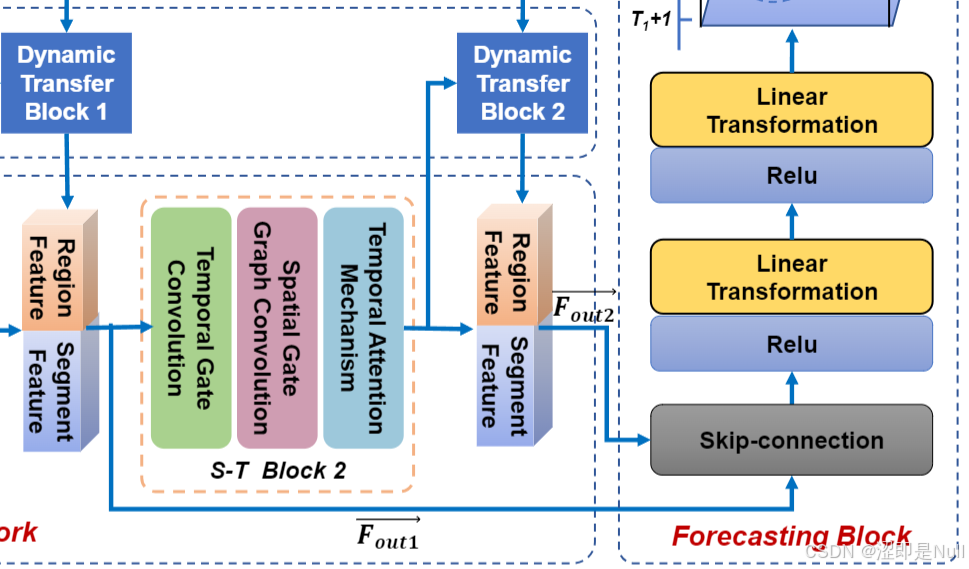
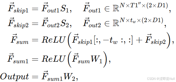
为从不同阶段的特征中提取更多信息，设计了跳跃连接（skip-connection）来汇聚上一步得到的两个不同特征，然后将汇聚结果输入预测模块。对比其他论文使用的残差网络（Res Net），残差连接的过程中加法操作是固定的，总是把原始信息无条件地加回来。而本篇论文使用的跳跃连接 + 动态传递模块则好比是一条"智能通道"，不仅传递原始信息，还会根据当前情况自动调节信息的"强度"。如果某部分信息更关键，它就会给它更大的权重；如果不那么重要，就会弱化它。

python 复制代码

self.skip_conv1 = Conv2d(2 * dilation_channels, skip_channels, kernel_size=(1, 1), stride=(1, 1), bias=True)
self.end_conv_1 = nn.Conv2d(in_channels=skip_channels, out_channels=end_channels, kernel_size=(1, 3), bias=True)
self.end_conv_2 = nn.Conv2d(in_channels=end_channels, out_channels=out_dim, kernel_size=(1, 1), bias=True)

s1 = self.skip_conv1(x)
skip = s1 + skip

# output
x = F.relu(skip)
x = F.relu(self.end_conv_1(x))
x = self.end_conv_2(x)