随着DeepSeek的火爆,AI大模型越来越被大众所接受,我们在日常生活和工作学习中也开始越来越频繁的使用豆包、通义千问、Kimi、DeepSeek、文心一言等大模型工具了。这些大模型底层技术都是Transformer模型,属于自然语言处理范畴。
今天开始,我们开始看看自然资源处理的原理。我参考的是斋藤康毅的《深度学习进阶:自然语言处理》。这次先讨论一下单词的表示和单词距离的计算方法。
一、概述
自然语言处理,英语简称NLP,通俗的讲,就是让计算机了解人类语言,然后完成对我们有用的事情。NLP可以做的事情很多,主要分为以下三类:
1.信息检索
自然语言处理技术可以用于改进搜索引擎。通过对用户输入的自然语言查询进行理解,搜索引擎可以更准确地找到相关的网页。例如,当用户输入 "如何制作巧克力蛋糕" 时,搜索引擎可以利用自然语言处理技术理解用户的意图是寻找制作巧克力蛋糕的方法,而不是巧克力蛋糕的历史等其他信息,从而提供更精准的搜索结果。
2.智能客服
智能客服系统利用自然语言处理技术来自动回答用户的问题。它可以理解用户的问题意图,并从知识库中检索相关信息进行回答。例如,在电商平台的客服系统中,当用户询问 "我购买的商品什么时候发货?" 时,智能客服可以自动回答发货时间等相关信息,提高客服效率。
3.文本分析和情感分析
在商业领域,自然语言处理可以用于分析社交媒体上的用户评论、产品评价等文本。情感分析可以判断文本的情感倾向是积极、消极还是中性。例如,企业可以通过分析用户对产品的评论,了解用户对产品的满意度,从而改进产品。对于电影评论,情感分析可以帮助电影制作方和发行方了解观众对电影的喜好程度。
自然语言处理处理主要的难度在于自然语言的多样性和歧义性。因为程序设计语言是高度规范化的语言,所以便于计算机处理,但是我们人类说的语言是各种各样的,而且很可能存在歧义,这就要依赖于不同的上下文。
自然语言处理的基础是语料库。语料库就是大量的文本数据。语料库中包含了大量的关于自然语言的实践知识,包括文章的写作方法,单词的选择方法,单词含义等。
二、分词
书中的例子是英语,为了更适合中文,我尝试用中文来实现。其实中文比英语更复杂,因为英语可以用单词作为基本单位,而中文是不能把单个文字作为基本语义单元的,因为中文至少要是一个词才可以表示一定的语义。所以我们需要先对一句话进行分词,这里就要借助一个python库------jieba。
jieba是一个中文分词库,可以很方便的对中文语句进行分词,得到一串词组。
python
import jieba

strs=["我来到北京清华大学","乒乓球拍卖完了","中国科学技术大学"]


for str in strs:
    seg_list = jieba.cut(str,use_paddle=True) # 使用paddle模式
    print("Paddle Mode: " + '/'.join(list(seg_list)))


seg_list = jieba.cut("我来到北京清华大学", cut_all=True)
print("全模式: " + "/ ".join(seg_list))  # 全模式


seg_list = jieba.cut("我来到北京清华大学", cut_all=False)
print("精确模式: " + "/ ".join(seg_list))  # 精确模式


seg_list = jieba.cut("他来到了网易杭研大厦")  # 默认是精确模式
print("新词识别:", ",".join(seg_list))

# 搜索引擎模式
seg_list = jieba.cut_for_search("小明硕士毕业于中国科学院计算所,后在日本京都大学深造")
print("搜索引擎模式: ", ",".join(seg_list))
# 输出:
Paddle Mode: 我/来到/北京/清华大学
Paddle Mode: 乒乓球/拍卖/完/了
Paddle Mode: 中国/科学技术/大学
全模式: 我/ 来到/ 北京/ 清华/ 清华大学/ 华大/ 大学
精确模式: 我/ 来到/ 北京/ 清华大学
新词识别: 他,来到,了,网易,杭研,大厦
搜索引擎模式:  小明,硕士,毕业,于,中国,科学,学院,科学院,中国科学院,计算,计算所,,,后,在,日本,京都,大学,日本京都大学,深造
我们这里使用默认的精确分词模式就可以了。假设我们有一句话:"小明今天去银泰双子楼看电影了"。我们可以对这句话进行分词,并看到几个单词的表示方式以及它们之间的距离。
python
seg_list = jieba.cut("小明今天去银泰双子楼看电影了")  # 默认是精确模式
print("新词识别:", "/".join(seg_list))
# 新词识别: 小明/今天/去/银泰/双子楼/看/电影/了
把得到的单词进行索引,赋予ID
python
word_to_id = {}
id_to_word = {}
seg_list = jieba.cut("小明今天去银泰双子楼看电影了")
words = list(seg_list)
for word in words:
    if word not in word_to_id:
        new_id = len(word_to_id)
        word_to_id[word] = new_id
        id_to_word[new_id] = word

print(word)
print(word_to_id)
# 输出
['小明', '今天', '去', '银泰', '双子楼', '看', '电影', '了']
{'小明': 0, '今天': 1, '去': 2, '银泰': 3, '双子楼': 4, '看': 5, '电影': 6, '了': 7}
可以看到,我们对每个单词赋予了一个ID,这个ID其实就是读到它们时的序号。我们把获取到语料库corpus,word_to_id和id_to_word的代码整合到一个函数中:
python
def preprocess(text):
    seg_list = jieba.cut(text)
    words = list(seg_list)
    word_to_id = {}
    id_to_word = {}
    for word in words:
        if word not in word_to_id:
            new_id = len(word_to_id)
            word_to_id[word] = new_id
            id_to_word[new_id] = word
    corpus = [word_to_id[w] for w in words]
    corpus = np.array(corpus)
    return corpus, word_to_id, id_to_word
三、单词的表示
在自然语言处理中,有个基本假设,单词的含义由它周围的单词形成。我们将上下文的大小成为窗口大小。在"小明今天去银泰双子楼看电影了"这句话中,如果窗口大小设置为1,"今天"的上下文就是"小明"和"去"。
我们把单词用共现矩阵来表示,所谓共现矩阵就是每行都是一个单词的上下文出现次数,如"今天"的共现次数就是1,0,1,0,0,0,0,0,因为"今天"的上下文只有"小明"和"去",所以这句话的共现矩阵如下所示:
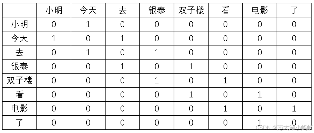
构建语料库的共现矩阵的代码如下:
python
def create_co_matrix(corpus, vocab_size, window_size=1):
    corpus_size = len(corpus)
    co_matrix = np.zeros((vocab_size, vocab_size), dtype=np.int32)
    for idx, word_id in enumerate(corpus):
        for i in range(1, window_size+1):
            left_idx = idx-i
            right_idx = idx+i

            if left_idx >= 0:
                left_word_id = corpus[left_idx]
                co_matrix[word_id, left_word_id] += 1

            if right_idx < corpus_size:
                right_word_id = corpus[right_idx]
                co_matrix[word_id, right_word_id] += 1

    return co_matrix

corpus, word_to_id, id_to_word = preprocess(text)
vocab_size = len(word_to_id)
C = create_co_matrix(corpus, vocab_size)


np.set_printoptions(precision=3) # 有效位数为3位
print('covariance matrix')
print(C)
# 输出:
covariance matrix
[[0 1 0 0 0 0 0 0]
 [1 0 1 0 0 0 0 0]
 [0 1 0 1 0 0 0 0]
 [0 0 1 0 1 0 0 0]
 [0 0 0 1 0 1 0 0]
 [0 0 0 0 1 0 1 0]
 [0 0 0 0 0 1 0 1]
 [0 0 0 0 0 0 1 0]]
四、单词相似度计算
通过共现矩阵表现了各个单词后,就可以计算单词之间的相似度了,常用的是余弦相似度,假设有两个向量x=(x1,x2,x3,...,xn)和y=(y1,y2,y3,...,yn)两个向量,他们之间的余弦相似度如下所示:
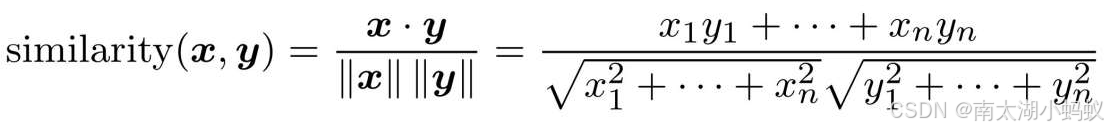
相似度计算代码如下,为了防止除数为0,所以加上一个微小值eps。
python
# 余弦相似度计算
# eps防止除数为0
def cos_similarity(x, y, eps=1e-8):
    nx = x/(np.sqrt(np.sum(x**2))+eps)
    ny = y/(np.sqrt(np.sum(y**2))+eps)
    return np.dot(nx, ny)
根据相似度计算的结果,可以对相似度进行排序,求得相似度比较高的单词
python
# 单词相似度排序函数
def most_similar(query, word_to_id, id_to_word, word_matrix, top=5):
    # 1.取出查询词
    if query not in word_to_id:
        print('%s is not found' % query)
        return
    print('\n[query] '+query)
    query_id = word_to_id[query]
    query_vec = word_matrix[query_id]

    # 2.计算余弦相似度
    vocab_size = len(id_to_word)
    similarity = np.zeros(vocab_size)
    for i in range(vocab_size):
        similarity[i] = cos_similarity(word_matrix[i], query_vec)

    # 3.基于余弦相似度,按降序输出值
    count = 0
    for i in (-1*similarity).argsort():
        if id_to_word[i] == query:
            continue
        print('%s : %s' % (id_to_word[i], similarity[i]))
        count += 1
        if count >= top:
            return

corpus, word_to_id, id_to_word = preprocess(text)
vocab_size = len(word_to_id)
C = create_co_matrix(corpus, vocab_size)


most_similar('去', word_to_id, id_to_word, C, top=5)
#输出:
[query] 去
小明 : 0.7071067691154799
双子楼 : 0.49999999292893216
今天 : 0.0
银泰 : 0.0
看 : 0.0
可以看到,"去"相似度最高的单词是"小明"和"双子楼",这也跟我们观察的结果一致。
书中还提到,如果仅仅是用这种共线矩阵来表示单词的相似度或者相关性,还有不合理的地方,比如英文中the和car,同时出现次数很高,但并不能表面the和car的相关性很强,所以改用了一种类似于条件概率的指标PMI来表示。
所谓的PMI,就是两次单词共同出现的次数除以两个单词各自出现次数的乘积,乘上语料库的大小,再求一下结果的对数,用公式表示就是:
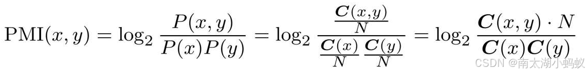
这个结果可以更加明确的表示两个单词之间的相似度。为了防止两个单词没有共同出现的时候,PMI结果会变成-∞,所以只取PMI>=0的结果。
python
def ppmi(C, verbose=False, eps=1e-8):
M = np.zeros_like(C, dtype=np.float32)
N = np.sum(C)
S = np.sum(C,axis=0)
total = C.shape[0] * C.shape[1]
cnt = 0
for i in range(C.shape[0]):
for j in range(C.shape[1]):
pmi = np.log2(C[i,j]*N/(S[j]*S[i])+eps)
M[i,j] = max(0, pmi)
return M
corpus, word_to_id, id_to_word = preprocess(text)
vocab_size = len(word_to_id)
C = create_co_matrix(corpus, vocab_size)
W = ppmi(C)
np.set_printoptions(precision=3) # 有效位数为3位
print('PPMI')
print(W)
# 输出:
PPMI
[[0. 2.807 0. 0. 0. 0. 0. 0. ]
[2.807 0. 1.807 0. 0. 0. 0. 0. ]
[0. 1.807 0. 1.807 0. 0. 0. 0. ]
[0. 0. 1.807 0. 1.807 0. 0. 0. ]
[0. 0. 0. 1.807 0. 1.807 0. 0. ]
[0. 0. 0. 0. 1.807 0. 1.807 0. ]
[0. 0. 0. 0. 0. 1.807 0. 2.807]
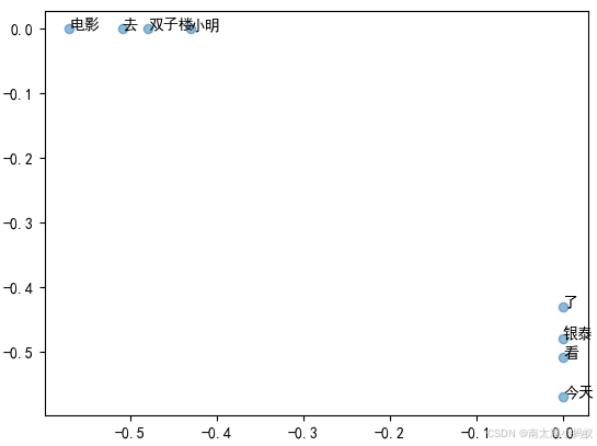
[0. 0. 0. 0. 0. 0. 2.807 0. ]]因为PMI矩阵比较稀疏,矩阵大量充斥着0,所以PMI矩阵可以通过奇异值分解,得到密集向量表示。
python
corpus, word_to_id, id_to_word = preprocess(text)
vocab_size = len(word_to_id)
C = create_co_matrix(corpus, vocab_size)
W = ppmi(C)

np.set_printoptions(precision=3) # 有效位数为3位
U,S,V = np.linalg.svd(W)
import matplotlib.pyplot as plt
plt.rcParams['font.sans-serif'] = 'SimHei' ## 设置字体为SimHei
plt.rcParams['axes.unicode_minus'] = False  ## 防止负号显示为一个方框

# 画出单词距离
for word, word_id in word_to_id.items():
    plt.annotate(word, (U[word_id,0], U[word_id,1]))

plt.scatter(U[:,0], U[:,1], alpha=0.5)
plt.show()
得到结果如下图:
五、实际案例
下面,我们使用一个复杂些的语料库来试试。假设我把《鬼吹灯3云南虫谷》的第一章文本作为语料库,我们来看看结果如何。
python
import jieba
# 导入《云南虫谷》第一章作为语料库
file_path = "D:\\zj\\AI\\云南虫谷第一章.txt"
words = open(file_path,encoding="utf-8").read().replace('\n', '<eos>').strip()

seg_list = jieba.cut(words)
words = list(seg_list)

word_to_id = {}
id_to_word = {}

for i, word in enumerate(words):
    if word not in word_to_id:
        tmp_id = len(word_to_id)
        word_to_id[word] = tmp_id
        id_to_word[tmp_id] = word


corpus = np.array([word_to_id[w] for w in words])
# 设置上下文窗口为2,词向量大小为100
window_size = 2
wordvec_size = 100

vocab_size = len(word_to_id)
print('counting co-occurrence...')
# 构建共现矩阵和PMI矩阵
C = create_co_matrix(corpus, vocab_size, window_size)
W = ppmi(C, verbose=True)
print('calculating SVD ...')

try:
    # 使用随机化算法计算矩阵的截断奇异值分解(SVD)
    from sklearn.utils.extmath import randomized_svd
    U,S,V = randomized_svd(W, n_components=wordvec_size, n_iter=5, random_state=None)
except ImportError:

    U,S,V = np.linalg.svd(W)
# 通过密集向量U获取词向量
word_vecs = U[:, :wordvec_size]
# 查看跟"金牙"相似度最高的几个词
querys = ['金牙']
for query in querys:
    most_similar(query, word_to_id, id_to_word, word_vecs, top=5)

#输出:
[query] 金牙
大 : 0.8146253824234009
事先 : 0.4061274528503418
凯旋归来 : 0.3681579530239105
杯中酒 : 0.35431432723999023
生意 : 0.352020263671875
可以看到"金牙"相似度最高的几个词,跟我们直观上的感觉是一致的,鬼吹灯中的"金牙"一般就是指奸商大金牙,"凯旋归来","生意"之类的都是大金牙的这段话的特质。可以用词云来看一下这段话:
python
# 停用词,过滤掉
stopwords = ["的","也","了"]


# 中文分词
file_path = "D:\\zj\\AI\\云南虫谷第一章.txt"
words = open(file_path,encoding="utf-8").read().replace('\n', '<eos>').strip()

seg_list = jieba.lcut(words)

processed_text = " ".join(seg_list)

# 去除停用词
filtered_words = [word for word in seg_list if word not in stopwords]

processed_text = " ".join(filtered_words)
# 创建词云对象
wordcloud = WordCloud(font_path='simhei.ttf', width=800, height=400, background_color='white').generate(processed_text)

# 设置图片清晰度
plt.rcParams['figure.dpi'] = 300

# 显示词云
plt.figure(figsize=(10, 5))
plt.imshow(wordcloud, interpolation='bilinear')
plt.axis('off')
plt.show()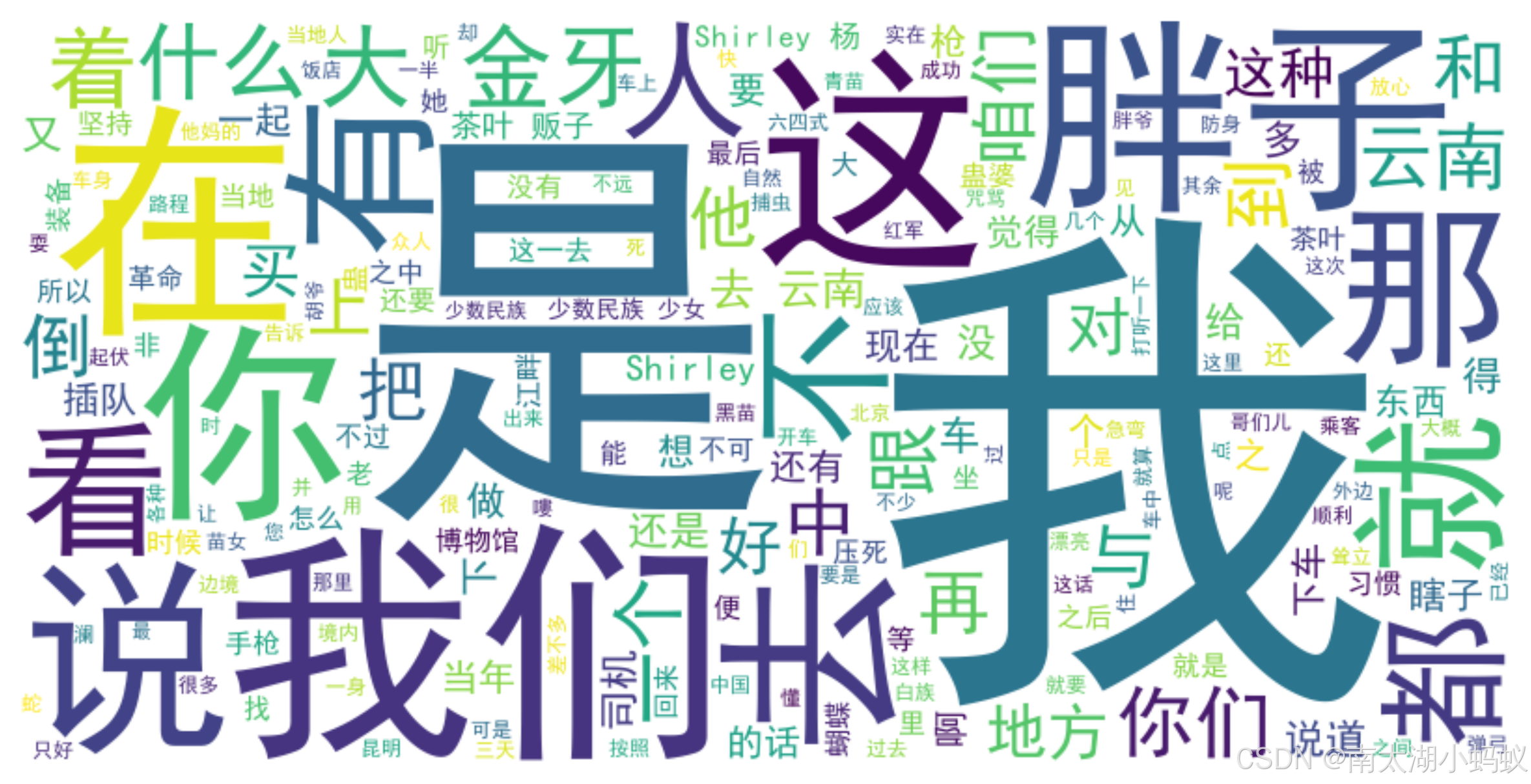
可以看到"胖子"和"大金牙"都很显眼,跟我们直观感觉是相符的。