目录
[1.1.torch.nn 核心模块](#1.1.torch.nn 核心模块)
1.神经网络
在 PyTorch 中 torch.nn 专门用于实现神经网络。其中 nn.Module 包含了网络层的搭建,以及一个方法-- forward(input) ,并返回网络的输出 outptu .
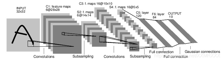
下面是一个经典的 LeNet 网络,用于对字符进行分类。
对于神经网络来说,一个标准的训练流程是这样的:⭐⭐⭐⭐⭐
- 定义一个多层的神经网络
- 对数据集的预处理并准备作为网络的输入
- 将数据输入到网络
- 计算网络的损失
- 反向传播,计算梯度
- 更新网络的梯度,一个简单的更新规则是 w= w - l* g
1.1.torch.nn 核心模块
基础层:
nn.Module:所有神经网络模块的基类,自定义网络必须继承此类。
python
import torch.nn as nn

class MyModel(nn.Module):
    def __init__(self):  # 注意:函数名应为__init__,而不是init
        super().__init__()  # 正确调用父类的__init__方法
        self.layer = nn.Linear(10, 5)  # 定义一个线性层,输入x:10,输出:5

    def forward(self, x):  # 定义前向传播函数
        return self.layer(x)  # 输入x通过线性层处理
nn.Sequential:顺序容器,简化层堆叠。
python
model = nn.Sequential(
    nn.Conv2d(1, 20, 5),
    nn.ReLU(),
    nn.Flatten()
)
常用层类型
- 线性层 :
nn.Linear(in_features, out_features) - 卷积层 :
nn.Conv2d(in_channels, out_channels, kernel_size) - 循环网络层 :
nn.LSTM(input_size, hidden_size, num_layers) - 归一化层 :
nn.BatchNorm2d(num_features)
激活函数
nn.ReLU()/nn.Sigmoid()/nn.Softmax(dim=1)
损失函数
- 分类任务:
nn.CrossEntropyLoss() - 回归任务:
nn.MSELoss() - 自定义损失:继承
nn.Module实现forward()
1.2.定义神经网络
首先定义一个神经网络,下面是一个 5 层的卷积神经网络,包含两层卷积层和三层全连接层:
python
import torch
import torch.nn as nn
import torch.nn.functional as F

class Net(nn.Module):

    def __init__(self):
        super(Net, self).__init__()
        # 输入图像是单通道,conv1 kenrnel size=5*5,输出通道 6
        self.conv1 = nn.Conv2d(1, 6, 5)
        # conv2 kernel size=5*5, 输出通道 16
        self.conv2 = nn.Conv2d(6, 16, 5)
        # 全连接层
        self.fc1 = nn.Linear(16*5*5, 120)
        self.fc2 = nn.Linear(120, 84)
        self.fc3 = nn.Linear(84, 10)

    def forward(self, x):
        # max-pooling 采用一个 (2,2) 的滑动窗口
        x = F.max_pool2d(F.relu(self.conv1(x)), (2, 2))
        # 核(kernel)大小是方形的话,可仅定义一个数字,如 (2,2) 用 2 即可
        x = F.max_pool2d(F.relu(self.conv2(x)), 2)
        x = x.view(-1, self.num_flat_features(x))
        x = F.relu(self.fc1(x))
        x = F.relu(self.fc2(x))
        x = self.fc3(x)
        return x

    def num_flat_features(self, x):
        # 除了 batch 维度外的所有维度
        size = x.size()[1:]
        num_features = 1
        for s in size:
            num_features *= s
        return num_features

net = Net()
print(net)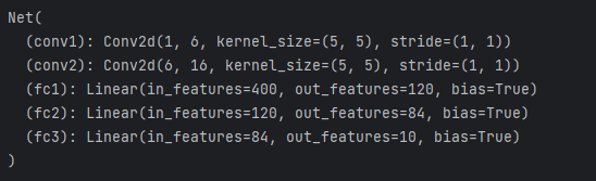
这里必须实现 forward 函数,而 backward 函数在采用 autograd 时就自动定义好了,在 forward 方法可以采用任何的张量操作。
net.parameters() 可以返回网络的训练参数,使用例子如下:
python
params = list(net.parameters())
print('参数数量: ', len(params))
# conv1.weight
print('第一个参数大小: ', params[0].size())
然后简单测试下这个网络,随机生成一个 32*32 的输入:
python
# 随机定义一个变量输入网络
input = torch.randn(1, 1, 32, 32)
out = net(input)
print(out)
input = torch.randn(1, 1, 32, 32)创建了一个形状为(1, 1, 32, 32)的张量。这个形状通常表示:
- 第一个维度(1):批次大小(batch size),即一次处理多少个图像。
- 第二个维度(1):通道数(channels),对于灰度图像是1,对于RGB图像是3。
- 第三个维度(32):图像的高度。
- 第四个维度(32):图像的宽度。
因此,这个张量代表了一个批次中包含的单个32x32像素的灰度图像。
接着反向传播需要先清空梯度缓存,并反向传播随机梯度:
python
# 清空所有参数的梯度缓存,然后计算随机梯度进行反向传播
net.zero_grad()
out.backward(torch.randn(1, 10))
torch.nn 只支持小批量(mini-batches)数据,也就是输入不能是单个样本,比如对于 nn.Conv2d 接收的输入是一个 4 维张量--nSamples * nChannels * Height * Width 。
所以,如果你输入的是单个样本,需要采用 input.unsqueeze(0) 来扩充一个假的 batch 维度,即从 3 维变为 4 维。
1.3.损失函数
损失函数的输入是 (output, target) ,即网络输出和真实标签对的数据,然后返回一个数值表示网络输出和真实标签的差距。
PyTorch 中其实已经定义了不少的损失函数,这里仅采用简单的均方误差:nn.MSELoss,例子如下:
python
output = net(input)
# 定义伪标签
target = torch.randn(10)
# 调整大小,使得和 output 一样的 size
target = target.view(1, -1)# 1*10
criterion = nn.MSELoss()

loss = criterion(output, target)
print(loss)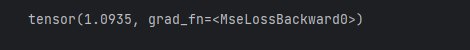
这里,整个网络的数据输入到输出经历的计算图如下所示,
input -> conv2d -> relu -> maxpool2d -> conv2d -> relu -> maxpool2d
调用 loss.backward() :
python
# MSELoss
print(loss.grad_fn)
# Linear layer
print(loss.grad_fn.next_functions[0][0])
# Relu
print(loss.grad_fn.next_functions[0][0].next_functions[0][0])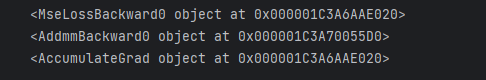
<MseLossBackward0 object at 0x000001C3A6AAE020>:
- 这是均方误差损失(MSELoss)的梯度函数。它用于计算损失函数关于其输入的梯度。在反向传播过程中,这个梯度函数会计算损失函数对输入的梯度。
<AddmmBackward0 object at 0x000001C3A70055D0>:
- 这是线性层(nn.Linear)的梯度函数。线性层的正向操作是
y = Ax + b,其中A是权重矩阵,x是输入,b是偏置。在反向传播过程中,这个梯度函数会计算关于权重、偏置和输入的梯度。
<AccumulateGrad object at 0x000001C3A6AAE020>:
- 这是用于累加梯度的梯度函数。在反向传播过程中,模型的参数(如权重和偏置)会累积梯度。这个梯度函数负责将计算出的梯度累加到相应的参数上。
1.4.反向传播
反向传播的实现只需要调用 loss.backward() 即可,当然首先需要清空当前梯度缓存,即.zero_grad() 方法,否则之前的梯度会累加到当前的梯度,这样会影响权值参数的更新。
下面是一个简单的例子,以 conv1 层的偏置参数 bias 在反向传播前后的结果为例:
python
# 清空所有参数的梯度缓存
net.zero_grad()
print('conv1.bias.grad before backward')
print(net.conv1.bias.grad)

loss.backward()

print('conv1.bias.grad after backward')
print(net.conv1.bias.grad)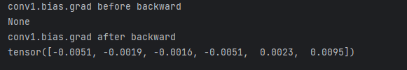
1.5.梯度更新
采用随机梯度下降(Stochastic Gradient Descent, SGD)方法的最简单的更新权重规则如下:
weight = weight - learning_rate * gradient
按照这个规则,代码实现如下所示:
python
# 简单实现权重的更新例子
learning_rate = 0.01
for f in net.parameters():#网络中所有可训练参数的迭代器,包括权重和偏置。
    f.data.sub_(f.grad.data * learning_rate)
遍历网络参数 :
net.parameters()返回网络中所有可训练参数的迭代器,包括权重和偏置。更新参数 :对于每个参数
f,其值通过减去f.grad.data * learning_rate来更新。这里:
f.data是参数的值。f.grad.data是参数的梯度,即在反向传播过程中计算出的梯度。sub_()是一个原地操作,用于直接在参数上减去给定的值,而不需要创建新的张量。
但是这只是最简单的规则,深度学习有很多的优化算法,不仅仅是 SGD,还有 Nesterov-SGD, Adam, RMSProp 等等,为了采用这些不同的方法,这里采用 torch.optim 库,使用例子如下所示:
python
import torch.optim as optim
# 创建优化器
optimizer = optim.SGD(net.parameters(), lr=0.01)

# 在训练过程中执行下列操作
optimizer.zero_grad() # 清空梯度缓存
output = net(input)
loss = criterion(output, target)
loss.backward()
# 更新权重
optimizer.step()注意,同样需要调用 optimizer.zero_grad() 方法清空梯度缓存。
2.图片分类器
在训练分类器前,当然需要考虑数据的问题。通常在处理如图片、文本、语音或者视频数据的时候,一般都采用标准的 Python 库将其加载并转成 Numpy 数组,然后再转回为 PyTorch 的张量。
·对于图像,可以采用 Pillow, OpenCV 库;
·对于语音,有 scipy 和 librosa;
·对于文本,可以选择原生 Python 或者 Cython 进行加载数据,或者使用 NLTK 和 SpaCy 。
PyTorch 对于计算机视觉,特别创建了一个 torchvision 的库,它包含一个数据加载器(data loader),可以加载比较常见的数据集,比如 Imagenet, CIFAR10, MNIST 等等,然后还有一个用于图像的数据转换器(data transformers),调用的库是 torchvision.datasets 和 torch.utils.data.DataLoader 。
在本教程中,将采用 CIFAR10 数据集,它包含 10 个类别,分别是飞机、汽车、鸟、猫、鹿、狗、青蛙、马、船和卡车。数据集中的图片都是 3x32x32。一些例子如下所示: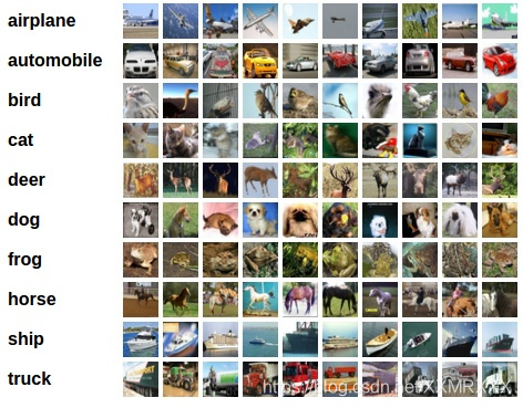
基础信息
- 全称:Canadian Institute For Advanced Research (CIFAR-10)
- 发布时间:2009年(至今仍是基准测试的黄金标准)
- 数据规模:60,000张32×32像素彩色图像(50k训练+10k测试)
- 类别分布:10类平衡数据,每类6,000张(含飞机、汽车、鸟类等常见物体)
训练流程如下:
- 通过调用 torchvision 加载和归一化 CIFAR10 训练集和测试集;
- 构建一个卷积神经网络;
- 定义一个损失函数;
- 在训练集上训练网络;
- 在测试集上测试网络性能。
2.1.数据加载
由于在pycharm中下载很慢,所以直接去官网下载,
官网下载:https://www.cs.toronto.edu/~kriz/cifar-10-python.tar.gz
python
import torch
import torchvision
import torchvision.transforms as transforms


# 定义数据预处理(含归一化到[-1,1])
transform = transforms.Compose([
    transforms.ToTensor(),
    transforms.Normalize((0.5, 0.5, 0.5), (0.5, 0.5, 0.5))
])

# 直接指向已下载的cifar-10-python文件夹
data_path = './data/cifar-10-python'  # 替换为实际路径

trainset = torchvision.datasets.CIFAR10(
    root=data_path,  # 关键修改:指定本地路径
    train=True,
    download=False,  # 禁用重复下载
    transform=transform
)
# 定义训练集数据加载器
trainloader = torch.utils.data.DataLoader(
    trainset,
    batch_size=4,# 批大小
    shuffle=True,# 是否打乱顺序
    num_workers=2# 多线程加载数据
)

# 定义测试集数据加载器
testset = torchvision.datasets.CIFAR10(
    root=data_path,  # 关键修改:指定本地路径
    train=False,
    download=False,  # 禁用重复下载
    transform=transform
    )
testloader = torch.utils.data.DataLoader(
    testset,
    batch_size=4,
    shuffle=False,
    num_workers=2
)
classes = ('plane', 'car', 'bird', 'cat',
           'deer', 'dog', 'frog', 'horse', 'ship', 'truck')
- transforms.
ToTensor():将PIL图像或NumPy数组转换为PyTorch张量(Tensor),格式为(C, H, W),自动将像素值从0, 255缩放到0.0, 1.0- transforms.Normalize
- 参数说明:
(mean_channels, std_channels)- 计算过程:
normalized = (input - mean) / stdtorchvision.datasets.CIFAR10():标准数据集接口
可视化数据:
python
from datetime import datetime
import matplotlib.pyplot  as plt
import torchvision
import numpy as np
from skimage import filters

def imshow_ultimate(img):
    # 预处理流程
    img = img / 2 + 0.5
    img_np = img.numpy().transpose(1,  2, 0)

    # 锐化+降噪
    img_np = filters.unsharp_mask(img_np,  radius=1, amount=1.8)

    # 可视化设置
    plt.figure(figsize=(15,  15), dpi=500)
    plt.imshow(img_np,
               interpolation='hanning',
               cmap='plasma',
               vmin=0.1, vmax=0.9)
    plt.axis('off')
    plt.title(f"CIFAR-10  Enhanced Preview\n{datetime.now().strftime('%Y-%m-%d  %H:%M')}")
    plt.show()

# 执行展示
dataiter = iter(trainloader)
images, labels = next(dataiter)
imshow_ultimate(torchvision.utils.make_grid(images[:4]))
print('清晰化标签:', ' | '.join(classes[labels[j]] for j in range(4)))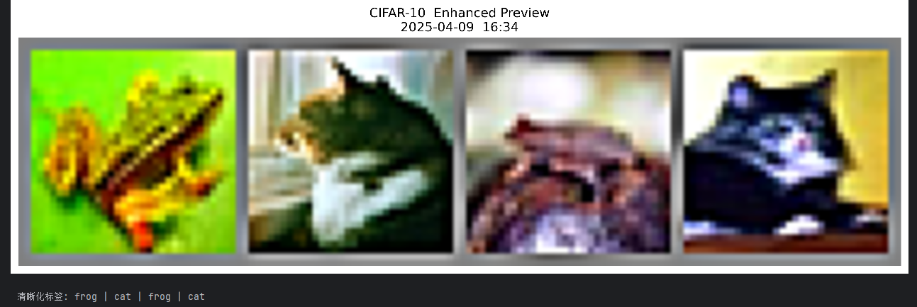
远古数据,可真的糊!!!!
2.2.卷积神经网络
python
import torch.nn as nn
import torch.nn.functional as F
class Net(nn.Module):
def __init__(self):
super(Net, self).__init__() # 调用父类nn.Module的初始化方法
# 第一卷积层:输入通道3(RGB),输出通道6,卷积核5x5(无padding默认valid卷积)
self.conv1 = nn.Conv2d(3, 6, 5)
# 最大池化层:窗口2x2,步长2(下采样率50%)
self.pool = nn.MaxPool2d(2, 2)
# 第二卷积层:输入通道6,输出通道16,卷积核5x5
self.conv2 = nn.Conv2d(6, 16, 5)
# 全连接层1:将16*5*5=400维特征映射到120维
self.fc1 = nn.Linear(16 * 5 * 5, 120)
# 全连接层2:120维到84维
self.fc2 = nn.Linear(120, 84)
# 输出层:84维到10维(对应CIFAR-10的10个类别)
self.fc3 = nn.Linear(84, 10)
def forward(self, x):
# 第一卷积块:Conv → ReLU → Pooling
x = self.pool(F.relu(self.conv1(x))) # 输出尺寸:6x14x14
# 第二卷积块:Conv → ReLU → Pooling
x = self.pool(F.relu(self.conv2(x))) # 输出尺寸:16x5x5
# 展平操作:将三维特征图转为一维向量(batch_size × 400)
x = x.view(-1, 16 * 5 * 5)
# 全连接层1 + ReLU激活
x = F.relu(self.fc1(x))
# 全连接层2 + ReLU激活
x = F.relu(self.fc2(x))
# 输出层(不接Softmax,因CrossEntropyLoss自带)
x = self.fc3(x)
return x
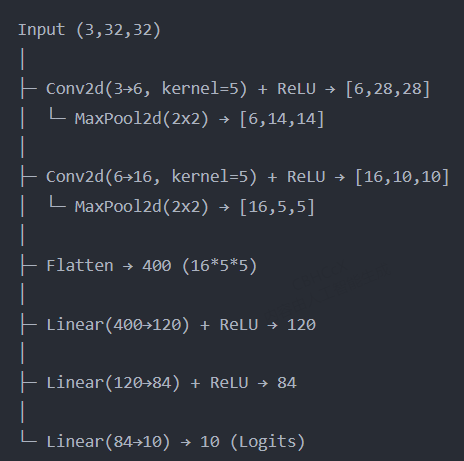
net = Net() 网络架构图:
2.3.优化器和损失
python
import torch.optim  as optim  # 导入优化器模块

criterion = nn.CrossEntropyLoss()

optimizer = optim.SGD(net.parameters(),  lr=0.001, momentum=0.9)
损失函数:交叉熵损失(适用于多分类任务)
特点:内部自动整合Softmax和Negative Log Likelihood
优化器:带动量的随机梯度下降(SGD)
参数说明:
- net.parameters(): 获取网络所有可训练参数
- lr=0.001: 学习率(2025年推荐初始值,需根据任务调整)
- momentum=0.9: 动量因子(加速收敛并减少震荡)
2.4.训练网络
指定需要迭代的 epoch,然后输入数据,指定次数打印当前网络的信息,比如 loss 或者准确率等性能评价标准。
python
import time
start = time.time()
for epoch in range(2):

    running_loss = 0.0
    for i, data in enumerate(trainloader, 0):
        # 获取输入数据
        inputs, labels = data
        # 清空梯度缓存
        optimizer.zero_grad()

        # 网络输出
        outputs = net(inputs)
        # 计算损失
        loss = criterion(outputs, labels)
        # 反向传播
        loss.backward()
        # 更新参数
        optimizer.step()

        # 打印统计信息
        running_loss += loss.item()
        if i % 2000 == 1999:
            # 每 2000 次迭代打印一次信息
            print('[%d, %5d] loss: %.3f' % (epoch + 1, i+1, running_loss / 2000))
            running_loss = 0.0
print('Finished Training! Total cost time in CPU: ', time.time()-start)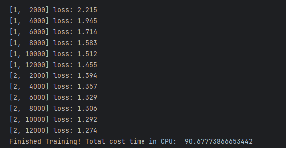
2.5.测试网络
训练好一个网络模型后,就需要用测试集进行测试,检验网络模型的泛化能力。对于图像分类任务来说,一般就是用准确率作为评价标准。
首先,我们先用一个 batch 的图片进行小小测试,这里 batch=4 ,也就是 4 张图片,代码如下:
python
dataiter = iter(testloader)
images, labels = next(dataiter)

# 打印图片
imshow_ultimate(torchvision.utils.make_grid(images))
print('GroundTruth: ', ' '.join('%5s' % classes[labels[j]] for j in range(4)))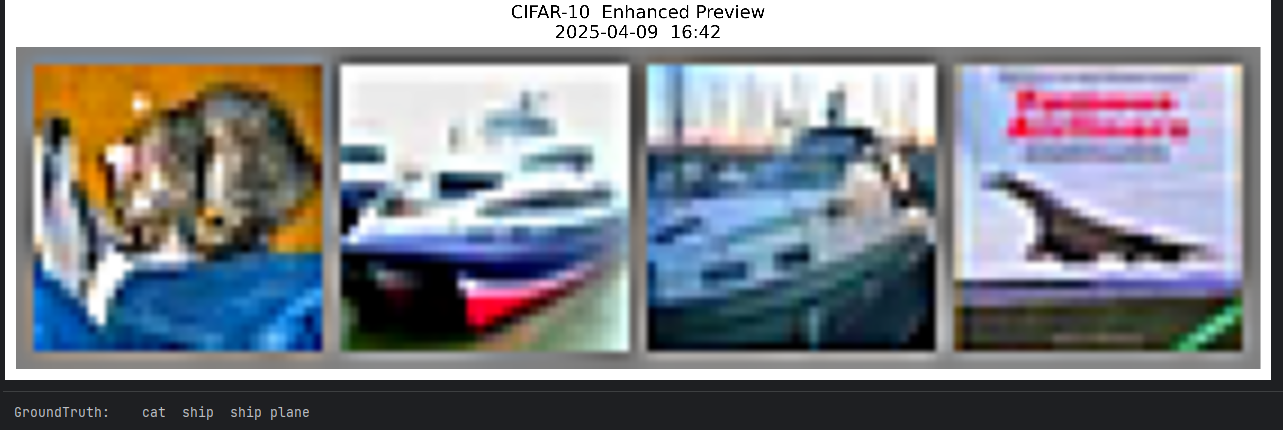
python
# 网络输出
outputs = net(images)

# 预测结果
_, predicted = torch.max(outputs, 1)
print('Predicted: ', ' '.join('%5s' % classes[predicted[j]] for j in range(4)))
前面三张图片都预测正确了,第四张图片错误预测飞机为船。
接着,让我们看看在整个测试集上的准确率可以达到多少吧!
python
correct = 0
total = 0
with torch.no_grad():
    for data in testloader:
        images, labels = data
        outputs = net(images)
        _, predicted = torch.max(outputs.data, 1)
        total += labels.size(0)
        correct += (predicted == labels).sum().item()

print('Accuracy of the network on the 10000 test images: %d %%' % (100 * correct / total))
python
class_correct = list(0. for i in range(10))
class_total = list(0. for i in range(10))
with torch.no_grad():
    for data in testloader:
        images, labels = data
        outputs = net(images)
        _, predicted = torch.max(outputs, 1)
        c = (predicted == labels).squeeze()
        for i in range(4):
            label = labels[i]
            class_correct[label] += c[i].item()
            class_total[label] += 1


for i in range(10):
    print('Accuracy of %5s : %2d %%' % (classes[i], 100 * class_correct[i] / class_total[i]))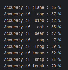
准确率差异:
- 数据层面问题
- 类别不平衡
- 示例:若
dog类训练样本仅100张,而ship类有5000张,模型会倾向预测高频类别。- 证据:
dog(7%)和bird(32%)准确率极低,可能样本量不足。- 标注噪声
- 低质量标注(如将
wolf误标为dog)会导致模型学习错误特征。- 特征相似性干扰
bird与plane(未出现类别)可能因蓝天背景混淆;deer与horse因四足形态相似易误判。
- 模型架构局限
- 浅层特征提取不足
- 若使用简单CNN(如LeNet),难以区分
cat/dog的细粒度纹理(如毛发vs皮毛)。- 过拟合特定类别
- 高准确率类别(如
ship81%)可能因训练集背景单一(如海景)导致模型依赖背景而非物体特征。
- 训练策略缺陷
- 损失函数未加权
- 默认交叉熵损失平等对待所有类别,加剧对小类别的忽略。
- 学习率/优化器不适配
- 固定学习率可能使模型快速收敛到主导类别(如
ship),忽略难样本(如dog)。
2.6.GPU上训练
python
device = torch.device("cuda:0" if torch.cuda.is_available() else "cpu")
print(device)

import time
# 在 GPU 上训练注意需要将网络和数据放到 GPU 上
net.to(device)
criterion = nn.CrossEntropyLoss()
optimizer = optim.SGD(net.parameters(), lr=0.001, momentum=0.9)

start = time.time()
for epoch in range(2):

    running_loss = 0.0
    for i, data in enumerate(trainloader, 0):
        # 获取输入数据
        inputs, labels = data
        inputs, labels = inputs.to(device), labels.to(device)
        # 清空梯度缓存
        optimizer.zero_grad()

        outputs = net(inputs)
        loss = criterion(outputs, labels)
        loss.backward()
        optimizer.step()

        # 打印统计信息
        running_loss += loss.item()
        if i % 2000 == 1999:
            # 每 2000 次迭代打印一次信息
            print('[%d, %5d] loss: %.3f' % (epoch + 1, i+1, running_loss / 2000))
            running_loss = 0.0
print('Finished Training! Total cost time in GPU: ', time.time() - start)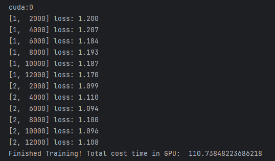
3.数据并行训练--多块GPU
这部分教程将学习如何使用 DataParallel 来使用多个 GPUs 训练网络。
首先,在 GPU 上训练模型的做法很简单,如下代码所示,定义一个 device 对象,然后用 .to() 方法将网络模型参数放到指定的 GPU 上。
python
device = torch.device("cuda:0")
model.to(device)
接着就是将所有的张量变量放到 GPU 上:
python
mytensor = my_tensor.to(device)注意,这里 my_tensor.to(device) 是返回一个 my_tensor 的新的拷贝对象,而不是直接修改 my_tensor 变量,因此你需要将其赋值给一个新的张量,然后使用这个张量。
Pytorch 默认只会采用一个 GPU,因此需要使用多个 GPU,需要采用 DataParallel ,代码如下所示:
python
model = nn.DataParallel(model)这代码也就是本节教程的关键。
3.1.导入和参数
python
import torch
import torch.nn as nn
from torch.utils.data import Dataset, DataLoader

# Parameters and DataLoaders
input_size = 5
output_size = 2

batch_size = 30
data_size = 100

device = torch.device("cuda:0" if torch.cuda.is_available() else "cpu")
定义网络输入大小和输出大小,batch 以及图片的大小,并定义了一个 device 对象。
3.2.构造一个虚拟数据集
接着就是构建一个假的(随机)数据集。实现代码如下:
python
class RandomDataset(Dataset):

    def __init__(self, size, length):
        self.len = length
        self.data = torch.randn(length, size)

    def __getitem__(self, index):
        return self.data[index]

    def __len__(self):
        return self.len

dataset=RandomDataset(input_size, data_size)
print(dataset[0:5])
rand_loader = DataLoader(dataset,
                         batch_size=batch_size,
                         shuffle=True)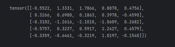
3.3.简单的网络
接下来构建一个简单的网络模型,仅仅包含一层全连接层的神经网络,加入 print() 函数用于监控网络输入和输出 tensors 的大小:
python
class Model(nn.Module):
    # Our model

    def __init__(self, input_size, output_size):
        super(Model, self).__init__()
        self.fc = nn.Linear(input_size, output_size)

    def forward(self, input):
        output = self.fc(input)
        print("\tIn Model: input size", input.size(),
              "output size", output.size())

        return output
3.4.创建数据并行
**⭐⭐⭐⭐⭐**定义一个模型实例,并且检查是否拥有多个 GPUs,如果是就可以将模型包裹在 nn.DataParallel ,并调用 model.to(device) 。代码如下:
python
model = Model(input_size, output_size)
if torch.cuda.device_count() >0:
  print("Let's use", torch.cuda.device_count(), "GPUs!")
  # dim = 0 [30, xxx] -> [10, ...], [10, ...], [10, ...] on 3 GPUs
  model = nn.DataParallel(model)

model.to(device)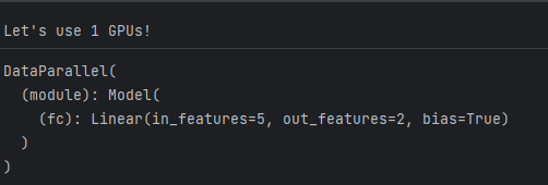
3.5.运行模型
接着就可以运行模型,看看打印的信息:
python
for data in rand_loader:
input = data.to(device)
output = model(input)
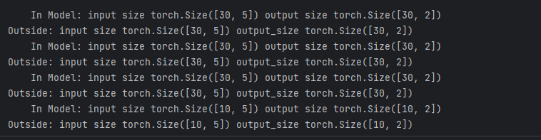
print("Outside: input size", input.size(),
"output_size", output.size())如果仅仅只有 1 个或者没有 GPU ,那么 batch=30 的时候,模型会得到输入输出的大小都是 30。但如果有多个 GPUs,那么结果如下:
2 GPUs
on 2 GPUs
Let's use 2 GPUs!
In Model: input size torch.Size(15, 5) output size torch.Size(15, 2)
In Model: input size torch.Size(15, 5) output size torch.Size(15, 2)
Outside: input size torch.Size(30, 5) output_size torch.Size(30, 2)
In Model: input size torch.Size(15, 5) output size torch.Size(15, 2)
In Model: input size torch.Size(15, 5) output size torch.Size(15, 2)
Outside: input size torch.Size(30, 5) output_size torch.Size(30, 2)
In Model: input size torch.Size(15, 5) output size torch.Size(15, 2)
In Model: input size torch.Size(15, 5) output size torch.Size(15, 2)
Outside: input size torch.Size(30, 5) output_size torch.Size(30, 2)
In Model: input size torch.Size(5, 5) output size torch.Size(5, 2)
In Model: input size torch.Size(5, 5) output size torch.Size(5, 2)
Outside: input size torch.Size(10, 5) output_size torch.Size(10, 2)
3 GPUs
Let's use 3 GPUs!
In Model: input size torch.Size(10, 5) output size torch.Size(10, 2)
In Model: input size torch.Size(10, 5) output size torch.Size(10, 2)
In Model: input size torch.Size(10, 5) output size torch.Size(10, 2)
Outside: input size torch.Size(30, 5) output_size torch.Size(30, 2)
In Model: input size torch.Size(10, 5) output size torch.Size(10, 2)
In Model: input size torch.Size(10, 5) output size torch.Size(10, 2)
In Model: input size torch.Size(10, 5) output size torch.Size(10, 2)
Outside: input size torch.Size(30, 5) output_size torch.Size(30, 2)
In Model: input size torch.Size(10, 5) output size torch.Size(10, 2)
In Model: input size torch.Size(10, 5) output size torch.Size(10, 2)
In Model: input size torch.Size(10, 5) output size torch.Size(10, 2)
Outside: input size torch.Size(30, 5) output_size torch.Size(30, 2)
In Model: input size torch.Size(4, 5) output size torch.Size(4, 2)
In Model: input size torch.Size(4, 5) output size torch.Size(4, 2)
In Model: input size torch.Size(2, 5) output size torch.Size(2, 2)
Outside: input size torch.Size(10, 5) output_size torch.Size(10, 2)
8 GPUs
Let's use 8 GPUs!
In Model: input size torch.Size(4, 5) output size torch.Size(4, 2)
In Model: input size torch.Size(4, 5) output size torch.Size(4, 2)
In Model: input size torch.Size(2, 5) output size torch.Size(2, 2)
In Model: input size torch.Size(4, 5) output size torch.Size(4, 2)
In Model: input size torch.Size(4, 5) output size torch.Size(4, 2)
In Model: input size torch.Size(4, 5) output size torch.Size(4, 2)
In Model: input size torch.Size(4, 5) output size torch.Size(4, 2)
In Model: input size torch.Size(4, 5) output size torch.Size(4, 2)
Outside: input size torch.Size(30, 5) output_size torch.Size(30, 2)
In Model: input size torch.Size(4, 5) output size torch.Size(4, 2)
In Model: input size torch.Size(4, 5) output size torch.Size(4, 2)
In Model: input size torch.Size(4, 5) output size torch.Size(4, 2)
In Model: input size torch.Size(4, 5) output size torch.Size(4, 2)
In Model: input size torch.Size(4, 5) output size torch.Size(4, 2)
In Model: input size torch.Size(4, 5) output size torch.Size(4, 2)
In Model: input size torch.Size(2, 5) output size torch.Size(2, 2)
In Model: input size torch.Size(4, 5) output size torch.Size(4, 2)
Outside: input size torch.Size(30, 5) output_size torch.Size(30, 2)
In Model: input size torch.Size(4, 5) output size torch.Size(4, 2)
In Model: input size torch.Size(4, 5) output size torch.Size(4, 2)
In Model: input size torch.Size(4, 5) output size torch.Size(4, 2)
In Model: input size torch.Size(4, 5) output size torch.Size(4, 2)
In Model: input size torch.Size(4, 5) output size torch.Size(4, 2)
In Model: input size torch.Size(4, 5) output size torch.Size(4, 2)
In Model: input size torch.Size(4, 5) output size torch.Size(4, 2)
In Model: input size torch.Size(2, 5) output size torch.Size(2, 2)
Outside: input size torch.Size(30, 5) output_size torch.Size(30, 2)
In Model: input size torch.Size(2, 5) output size torch.Size(2, 2)
In Model: input size torch.Size(2, 5) output size torch.Size(2, 2)
In Model: input size torch.Size(2, 5) output size torch.Size(2, 2)
In Model: input size torch.Size(2, 5) output size torch.Size(2, 2)
In Model: input size torch.Size(2, 5) output size torch.Size(2, 2)
Outside: input size torch.Size(10, 5) output_size torch.Size(10, 2
DataParallel 会自动分割数据集并发送任务给多个 GPUs 上的多个模型。然后等待每个模型都完成各自的工作后,它又会收集并融合结果,然后返回。