深度学习3.1 线性回归

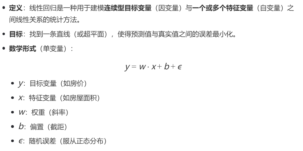
3.1.1 线性回归的基本概念

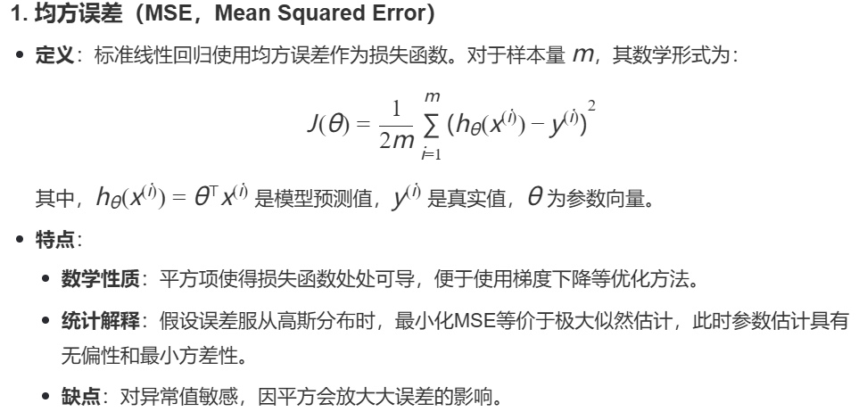
损失函数

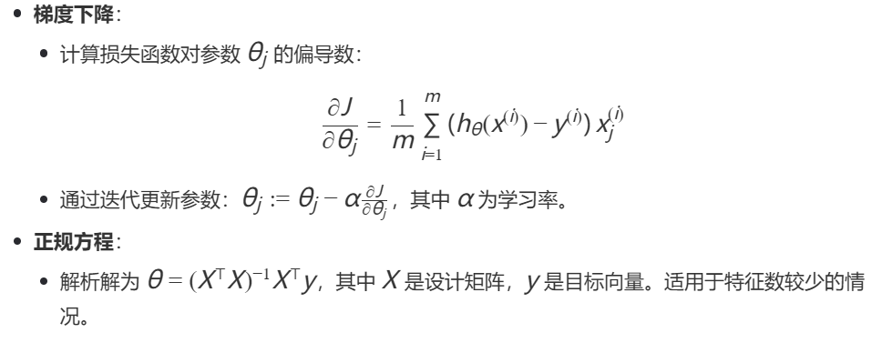
梯度下降

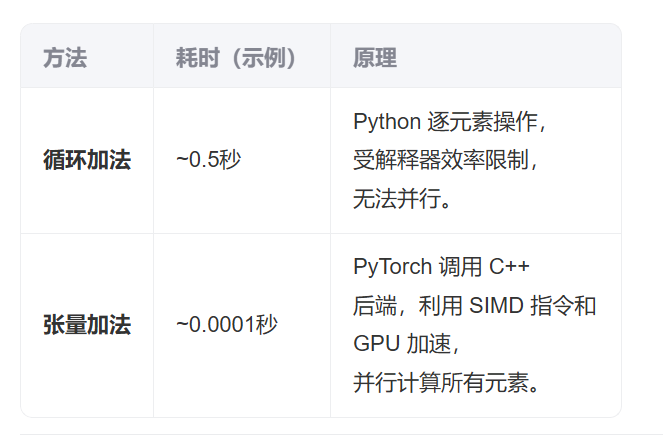
3.1.2 向量化加速

python 复制代码

%matplotlib inline
import math
import time
import numpy as np
import torch
from d2l import torch as d2l

n = 1000000 #本机为了差距明显，选择数据较大，运行时间较长，可选择10000
a = torch.ones(n)
b = torch.ones(n)


class Timer:
    def __init__(self):
        self.times = []  # 存储每次测量的时间
        self.start()      # 初始化时自动开始计时

    def start(self):
        self.tik = time.time()  # 记录当前时间戳（开始时间）

    def stop(self):
        self.times.append(time.time() - self.tik)  # 计算并保存时间差
        return self.times[-1]  # 返回本次测量的时间

    def avg(self):
        return sum(self.times) / len(self.times)  # 平均耗时

    def sum(self):
        return sum(self.times)  # 总耗时

    def cumsum(self):
        return np.array(self.times).cumsum().tolist()  # 累计耗时（用于绘图）

python 复制代码

c = torch.zeros(n)      # 初始化全0张量 c（存储结果）
timer = Timer()         # 创建计时器实例
for i in range(n):
    c[i] = a[i] + b[i]  # 逐个元素相加（慢！）
print(f'{timer.stop():.5f} sec')

'19.59485 sec'

python 复制代码

timer.start()
d = a + b
f'{timer.stop():.5f} sec'

'0.00470 sec'

3.1.3 正态分布与平方损失

python 复制代码

import math
import numpy as np
from d2l import torch as d2l

def normal(x, mu, sigma):
    p = 1 / math.sqrt(2 * math.pi * sigma ** 2)  # 归一化系数
    return p * np.exp(-0.5 / sigma ** 2 * (x - mu) ** 2)  # 概率密度计算

x = np.arange(-7, 7, 0.01)  # 生成 [-7, 7) 区间内步长0.01的数组
params = [(0, 1), (0, 2), (3, 1)]  # (mu, sigma) 的组合 (均值, 标准差)

d2l.plot(
    x,  # x 轴数据
    [normal(x, mu, sigma) for mu, sigma in params],  # y 轴数据列表（三条曲线）
    xlabel='x',  # x 轴标签
    ylabel='p(x)',  # y 轴标签
    figsize=(4.5, 2.5),  # 图像尺寸（宽，高）
    legend=[f'mean {mu}, std {sigma}' for mu, sigma in params]  # 图例说明
)

深度学习3.1 线性回归

3.1.1 线性回归的基本概念

损失函数

梯度下降

3.1.2 向量化加速

3.1.3 正态分布与平方损失

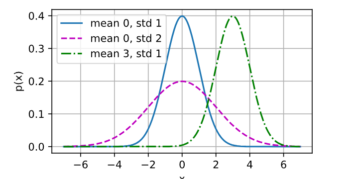
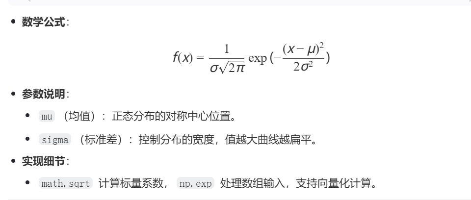
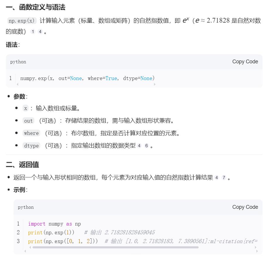
x 是 NumPy 数组，np.exp 支持数组运算，而 math.exp 仅处理标量。