Mip-Splatting: Alias-free 3D Gaussian Splatting
论文地址:https://arxiv.org/abs/2403.17888
源码地址:https://github.com/autonomousvision/mip-splatting
项目地址:https://niujinshuchong.github.io/mip-splatting/
论文解读
- 两个主要贡献点, 一个3D滤波器,一个2D滤波器
- 3D滤波主要约束3D高斯的高频频率
- 2D滤波主要解决屏幕投影的膨胀和失真问题
- 这个方法对场景细节应该会有优化,可以去除细节处的毛刺和floater
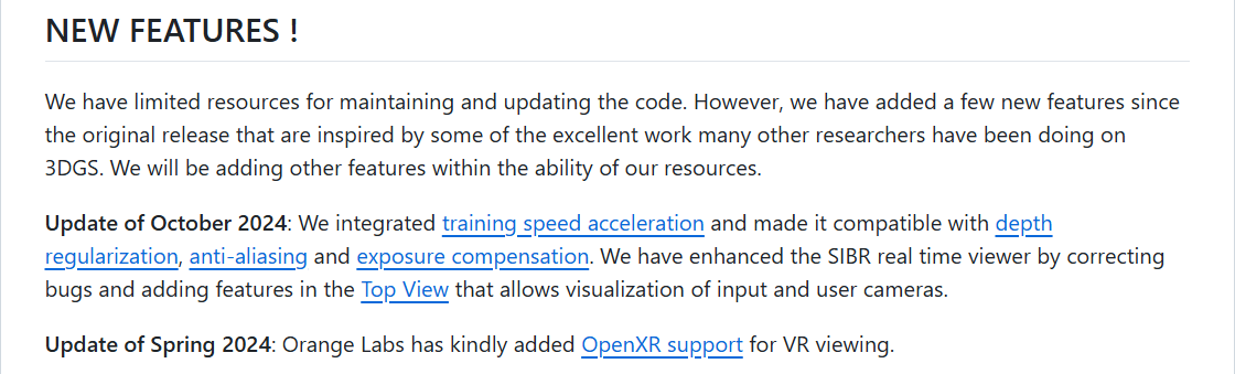
- 3DGS在最近的feature更新中加入了这一特性,大家也可以参考
3D滤波器
compute_3D_filter函数计算出需要最大采样频率 ν ^ k \hat{\nu}_k ν^k和采样间隔 T ^ \hat{T} T^,论文中更新滤波器的频次和致密化的频率是一致的
python
  @torch.no_grad()
  def compute_3D_filter(self, cameras):
    print("Computing 3D filter")
    #TODO consider focal length and image width
    xyz = self.get_xyz
    distance = torch.ones((xyz.shape[0]), device=xyz.device) * 100000.0
    valid_points = torch.zeros((xyz.shape[0]), device=xyz.device, dtype=torch.bool)

    # we should use the focal length of the highest resolution camera
    focal_length = 0.
    for camera in cameras:

      # transform points to camera space
      R = torch.tensor(camera.R, device=xyz.device, dtype=torch.float32)
      T = torch.tensor(camera.T, device=xyz.device, dtype=torch.float32)
      # R is stored transposed due to 'glm' in CUDA code, so we don't neet transpose here
      xyz_cam = xyz @ R + T[None, :]

      xyz_to_cam = torch.norm(xyz_cam, dim=1)

      # project to screen space
      valid_depth = xyz_cam[:, 2] > 0.2

      x, y, z = xyz_cam[:, 0], xyz_cam[:, 1], xyz_cam[:, 2]
      z = torch.clamp(z, min=0.001)

      x = x / z * camera.focal_x + camera.image_width / 2.0
      y = y / z * camera.focal_y + camera.image_height / 2.0

      # in_screen = torch.logical_and(torch.logical_and(x >= 0, x < camera.image_width), torch.logical_and(y >= 0, y < camera.image_height))

      # use similar tangent space filtering as in the paper
      in_screen = torch.logical_and(torch.logical_and(x >= -0.15 * camera.image_width, x <= camera.image_width * 1.15),
                                    torch.logical_and(y >= -0.15 * camera.image_height,y <= 1.15 * camera.image_height))

      valid = torch.logical_and(valid_depth, in_screen)

      # distance[valid] = torch.min(distance[valid], xyz_to_cam[valid])
      distance[valid] = torch.min(distance[valid], z[valid])
      valid_points = torch.logical_or(valid_points, valid)
      if focal_length < camera.focal_x:
        focal_length = camera.focal_x
		# 对应论文公式7
    distance[~valid_points] = distance[valid_points].max()

    #TODO remove hard coded value
    #TODO box to gaussian transform
    #todo:对应公式6,但是这个系数哪里有说明?
    filter_3D = distance / focal_length * (0.2 ** 0.5)
self.filter_3D = filter_3D[..., None]- 3D滤波应用在scale和opacity两个高斯属性上面
python
    @property
  def get_scaling_with_3D_filter(self):
    scales = self.get_scaling

    scales = torch.square(scales) + torch.square(self.filter_3D)
    scales = torch.sqrt(scales)
    return scales

  @property
  def get_opacity_with_3D_filter(self):
    # todo:对应公式9
    opacity = self.opacity_activation(self._opacity)
    # apply 3D filter
    scales = self.get_scaling
		# scale是[N,3,1]的张量,可以通过平方和prod得到对角矩阵的行列式
    scales_square = torch.square(scales)
    det1 = scales_square.prod(dim=1)

    scales_after_square = scales_square + torch.square(self.filter_3D)
    det2 = scales_after_square.prod(dim=1)
    coef = torch.sqrt(det1 / det2)
return opacity * coef[..., None]关于opacity校正的部分,在repo的issue48中有深入讨论:从理论上这里对opacity的处理是有问题的,本身3D滤波不应该对不透明度进行处理,应该只对scale进行限制。但是作者实验之后发现还是存在一定的floater;问题提出人给出了实验结果,但是这种处理会增加很多的高斯,我猜测是因为限制scale之后导致整体环境的表示需要更多的高斯去拟合,导致了ply数量的增长;
- 3D滤波器选择方差(kernel size)为0.2和2D滤波的方差0.1是为了保证组合效果,作者在实验后测试的结果;
2D滤波器
- 代码实现,这里是在render的cuda算子中进行了实现;目前有人在gsplat上面进行的尝试,链接在这里
cpp
// Forward version of 2D covariance matrix computation
__device__ float4 computeCov2D(const float3& mean, float focal_x, float focal_y, float tan_fovx, float tan_fovy, float kernel_size, const float* cov3D, const float* viewmatrix)
{
	// The following models the steps outlined by equations 29
	// and 31 in "EWA Splatting" (Zwicker et al., 2002).
	// Additionally considers aspect / scaling of viewport.
	// Transposes used to account for row-/column-major conventions.
	float3 t = transformPoint4x3(mean, viewmatrix);

	const float limx = 1.3f * tan_fovx;
	const float limy = 1.3f * tan_fovy;
	const float txtz = t.x / t.z;
	const float tytz = t.y / t.z;
	t.x = min(limx, max(-limx, txtz)) * t.z;
	t.y = min(limy, max(-limy, tytz)) * t.z;

	glm::mat3 J = glm::mat3(
		focal_x / t.z, 0.0f, -(focal_x * t.x) / (t.z * t.z),
		0.0f, focal_y / t.z, -(focal_y * t.y) / (t.z * t.z),
		0, 0, 0);

	glm::mat3 W = glm::mat3(
		viewmatrix[0], viewmatrix[4], viewmatrix[8],
		viewmatrix[1], viewmatrix[5], viewmatrix[9],
		viewmatrix[2], viewmatrix[6], viewmatrix[10]);

	glm::mat3 T = W * J;

	glm::mat3 Vrk = glm::mat3(
		cov3D[0], cov3D[1], cov3D[2],
		cov3D[1], cov3D[3], cov3D[4],
		cov3D[2], cov3D[4], cov3D[5]);

	glm::mat3 cov = glm::transpose(T) * glm::transpose(Vrk) * T;

	// Apply low-pass filter: every Gaussian should be at least
	// one pixel wide/high. Discard 3rd row and column.
	// compute the coef of alpha based on the detemintant, 对应论文公式10
	const float det_0 = max(1e-6, cov[0][0] * cov[1][1] - cov[0][1] * cov[0][1]);
	const float det_1 = max(1e-6, (cov[0][0] + kernel_size) * (cov[1][1] + kernel_size) - cov[0][1] * cov[0][1]);
	float coef = sqrt(det_0 / (det_1+1e-6) + 1e-6);

	if (det_0 <= 1e-6 || det_1 <= 1e-6){
		coef = 0.0f;
	}
  // kernel_size=0.1, 原版3DGS这里是0.3
	cov[0][0] += kernel_size;
	cov[1][1] += kernel_size;

	return { float(cov[0][0]), float(cov[0][1]), float(cov[1][1]), float(coef)};
}-
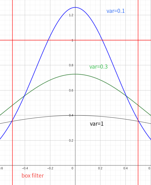
kernel_size设定为0.1,这里的链接解释了为什么选择0.1作为高斯分布的方差,和论文中阐述是一致的,主要是模拟了一个box filter,理想情况是值用1个像素内的分布,0.1的高斯分布是最接近box filter的;下图表示了不同方差对应高斯分布;在最终的数据表现上,0.1的方差效果更好,细节处应该是表现更优秀的,但是会导致更多的高斯球,这对显存和训练耗时是个挑战;
-
VanlliaGS中也对去毛刺的方案进行了实现,但是将kernel_size设置为0.3;
Reference
对采样定理的浅显解释
- 采样定理的Wiki:https://zh.wikipedia.org/zh-cn/采样定理
Nyquist-Shannon采样定理是信号处理领域的一项基本原理。它说明了如何从连续信号中准确重构离散信号。
基本概念
- 连续信号:原始的模拟信号,通常随时间连续变化。
- 离散信号(采样信号):对连续信号依照一定间隔进行采样得到的数值集合。
采样定理内容
- 采样率 :采样信号的频率,即每秒对连续信号进行采样的次数,用 f s f_s fs表示。
- 最大频率(带宽) :连续信号中包含的最高频率成分,用 f m a x f_{max} fmax表示。
定理 :要从采样信号中完全重建原始信号,采样率必须大于两倍的最大频率: f s > 2 × f m a x f_s > 2 \times f_{max} fs>2×fmax
这个条件也称为奈奎斯特频率 (Nyquist Frequency),即: f s = 2 × f m a x f_s = 2 \times f_{max} fs=2×fmax
实际意义
- 防止混叠(Aliasing):若采样率过低,信号中的高频成分将无法被正确重建,产生混叠现象,使不同频率的信号在重建时混淆在一起。
- 信号重构:在满足Nyquist频率的条件下,可以使用适当的滤波器(如低通滤波器)从采样数据中完美重构原始信号。
应用实例
- 音频处理:CD音频的采样率通常为44.1 kHz,超过人类可听频率(约20 kHz)的两倍,以确保音质。
- 图像处理:屏幕显示时,需要针对像素密度来选择适当的采样率以防止视觉伪影。
总结
Nyquist-Shannon采样定理为信号处理中的离散化提供了理论基础,指导如何选择适当的采样率来确保信号的完整重建。这对于数字音频、图像及通信系统等领域至关重要。