本文将展示YOLOv8中损失函数计算的完整代码解析,注释中提供了详尽的解释,并结合示例演示了数据维度的转换,以帮助更好地理解。
YOLOv8的损失函数计算代码位于'ultralytics/utils/loss.py'文件中(如下所示),我在代码中的注释提供了详细解析。
首先看一下整体包含哪些方法
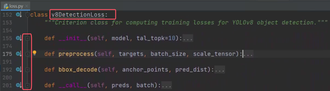
__init__和preprocess的代码如下
python
class v8DetectionLoss:
"""Criterion class for computing training losses for YOLOv8 object detection."""
def __init__(self, model, tal_topk=10): # model must be de-paralleled
"""Initialize v8DetectionLoss with model parameters and task-aligned assignment settings."""
# 获取模型的设备信息(模型参数所在的设备 CPU/GPU)
device = next(model.parameters()).device # get model device
# 获取模型的超参数配置(如超参数字典,包含损失权重等)
h = model.args # hyperparameters
# 获取模型最后一层,一般是 Detect() 模块,其中包含输出相关的属性
m = model.model[-1] # Detect() module
# 定义二元交叉熵损失(带Logits版),用于分类损失计算(reduction="none"表示不在内部求和,保留逐元素损失)
self.bce = nn.BCEWithLogitsLoss(reduction="none")
# 保存超参数配置到属性 hyp,以便后续使用(例如获取损失权重)
self.hyp = h
# 模型的步长列表,每个输出层相对于原图的下采样倍数
self.stride = m.stride # model strides
# 模型的类别数(number of classes)
self.nc = m.nc # number of classes
# 输出通道数 no = 类别数 + 每个边界框预测的分布参数数目 (reg_max * 4)
# 例如,如果类别数 nc=80,reg_max=16,则 no = 80 + 16*4 = 144
self.no = m.nc + m.reg_max * 4
# 每个边界框回归的最大分布区间(reg_max,一般用于分布Focal Loss)
self.reg_max = m.reg_max
# 保存设备信息到属性 device
self.device = device
# 标志是否使用 DFL(Distribution Focal Loss),当 reg_max > 1 时使用
self.use_dfl = m.reg_max > 1
# 初始化任务对齐分配器(Task-Aligned Assigner),用于在训练时匹配预测和真实目标
self.assigner = TaskAlignedAssigner(topk=tal_topk, num_classes=self.nc, alpha=0.5, beta=6.0)
# 初始化边界框损失函数(BboxLoss),传入 reg_max,用于计算边界框的回归损失(如 IoU 和 DFL)
self.bbox_loss = BboxLoss(m.reg_max).to(device)
# 创建投影张量 self.proj,用于将分布转换为具体距离(值为0,1,...,reg_max-1),放在与模型相同的设备上
self.proj = torch.arange(m.reg_max, dtype=torch.float, device=device)
def preprocess(self, targets, batch_size, scale_tensor):
"""
预处理目标数据:转换为张量格式并缩放坐标
模型需要固定形状的输入(如 (batch_size, N, 5)),而原始标注的目标数量是动态的。
比如targets中的nl(总目标数),不同batch中的总目标数不一样,预测的结果难以统一。
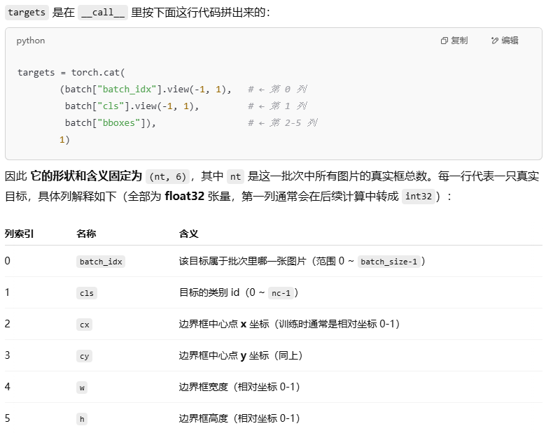
targets 是在 __call__ 里用concat拼出来的:
参数:
targets: 原始标注数据,形状为(nl, ne),其中
nl = 当前batch的总目标数
ne = [batch_index, class_id, x_center, y_center, width, height]
batch_size: 当前batch的样本数
scale_tensor: 缩放因子(用于将归一化坐标还原为输入图像尺度)
示例输入:
batch_size=2
targets = [
[0, 3, 0.5, 0.5, 0.2, 0.3], # 图像0中的目标
[0, 1, 0.3, 0.4, 0.1, 0.2],
[1, 5, 0.7, 0.8, 0.2, 0.1] # 图像1中的目标
]
scale_tensor = tensor([640, 640, 640, 640])(假设输入图像尺寸为640x640)
"""
nl, ne = targets.shape
if nl == 0: # 如果当前batch没有目标
'''
out是预处理后的目标张量,其形状为: (batch_size, max_targets_per_image, 5)
其中:
batch_size:当前批次的图像数量(例如2)。
max_targets_per_image:当前批次中单张图像的最大目标数量(例如10)。
5: 每个目标的属性,格式为 [class_id, x_min, y_min, x_max, y_max]。
'''
out = torch.zeros(batch_size, 0, ne - 1, device=self.device)
else:
i = targets[:, 0] # 取出了所有真实框的图像索引列,方便按图像分组统计。
# 计算每个图像的目标数
# 对一维张量i做去重,并计算每个唯一值出现的次数。counts里的每个元素就是对应那张图像有多少个真实框。
_, counts = i.unique(return_counts=True)
counts = counts.to(dtype=torch.int32)
# 创建输出张量:形状为(batch_size, max_counts, ne-1)
# 示例:当max_counts=2时,形状为(2, 2, 5)
out = torch.zeros(batch_size, counts.max(), ne - 1, device=self.device)
# 按图像填充数据
for j in range(batch_size):
'''
例:假设 batch_size=3 且
i = tensor([0, 0, 1, 2, 2]) # 5 个框
• 当 j = 0 :
matches = tensor([ True, True, False, False, False])
• 当 j = 1 :
matches = tensor([False, False, True, False, False])
• 当 j = 2 :
matches = tensor([False, False, False, True, True ])
matches 是一个布尔张量,标记哪些目标属于第 j 张图像
'''
matches = i == j
if n := matches.sum(): # 该图像有n个目标
# 将匹配的目标数据存入out[j],去除第一列(图像索引)
# 示例:当j=0时,存入前两个目标的[3,0.5,0.5,0.2,0.3]和[1,0.3,0.4,0.1,0.2]
out[j, :n] = targets[matches, 1:] # [max_counts, 5]
# 将坐标从归一化的xywh转换为图像尺度的xyxy
# out[..., 1:5]形状:(batch_size, max_counts, 4)
# 示例转换前:[[0.5,0.5,0.2,0.3], ...] 归一化的xywh
# 转换后得到绝对坐标:[[320, 320, 192, 384], ...]
out[..., 1:5] = xywh2xyxy(out[..., 1:5].mul_(scale_tensor))
return out # 输出形状:(batch_size, max_counts, 5)上面代码中的targets来源如下
bbox_decode代码如下:
python
def bbox_decode(self, anchor_points, pred_dist):
    """
    将网络输出的 **距离分布(pred_dist)** 解码成最终的边界框坐标 (x1,y1,x2,y2)。

    ─────────────────────────────────────────────────────────────
    ✦ 参数说明
    ----------------------------------------------------------------
      anchor_points : Tensor(shape=(A, 2))
          → 每个输出位置(=anchor) 在特征图上的中心点坐标 (cx, cy),已按 stride
            归一化到与 pred_dist 同尺度;A=全部输出点总数 (H₁W₁+H₂W₂+...)
      pred_dist     : Tensor(shape=(B, A, 4*reg_max))
          → 模型回归头直接输出的 **离散距离分布**:
             对于每个 anchor,一共 4 个方向(左、上、右、下),
             每个方向用 reg_max 个 bin 表示离地的概率分布。

      例:batch_size(B)=2,A=8400,reg_max=16
           ⇒ pred_dist.shape = (2, 8400, 4*16=64)

    ✦ 返回值
      Tensor(shape=(B, A, 4))   # 对应每个 anchor 的 [l, t, r, b] 像素距离
    ─────────────────────────────────────────────────────────────
    """

    # 1) 如果使用 Distribution Focal Loss(DFL) ------ reg_max > 1
    if self.use_dfl:                            # True 当 reg_max > 1
        b, a, c = pred_dist.shape               # b=B, a=A, c=4*reg_max
        # ---------- ① view ----------
        # 把 "channel = 4*reg_max" 拆成 "4 个方向 × reg_max bins"
        # (B, A, 64)  →  (B, A, 4, 16)
        pred_dist = pred_dist.view(b, a, 4, c // 4)

        # ---------- ② softmax ----------
        # 对最后一维(16)做 softmax → 获得离散概率分布
        pred_dist = pred_dist.softmax(3)

        # ---------- ③ 期望值 (matmul) ----------
        # self.proj = tensor([0,1,2,...,15])  ← shape (16,)
        # 期望 = Σ p_k * k
        # 形状推导:
        #   (B, A, 4, 16)  @  (16,)  →  (B, A, 4)
        pred_dist = pred_dist.matmul(self.proj.type(pred_dist.dtype))

        # ⚠️ 此时 pred_dist 的含义已经从"概率分布"→"具体距离值(左,上,右,下)"

        # ▼ 小示例(单 anchor)------------------------------------
        #    假设 reg_max=4, softmax 结果 = [0.1, 0.2, 0.6, 0.1]
        #    self.proj = [0, 1, 2, 3]
        #    距离 = 0*0.1 + 1*0.2 + 2*0.6 + 3*0.1 = 1.7
        # --------------------------------------------------------

    # 2) 将 "距离格式(l,t,r,b)" 转成 "bbox 坐标(x1,y1,x2,y2)"
    #    dist2bbox 内部做:x1 = cx - l   ,  y1 = cy - t
    #                     x2 = cx + r   ,  y2 = cy + b
    #    如果 xywh=False ⇒ 返回 xyxy
    bboxes = dist2bbox(pred_dist,                # (B, A, 4)  距离
                       anchor_points,            # (A, 2)     锚点中心
                       xywh=False)               # ← 输出 xyxy

    return bboxes
形状与数据流全览(以 B=2, A=8400, reg_max=16 为例)
| 步骤 | 张量名 | 形状 | 备注 |
|---|---|---|---|
| 输入 | pred_dist |
(2, 8400, 64) |
每点 64 通道 = 4×16 |
| ① | view |
(2, 8400, 4, 16) |
拆成 4 方向 × 16 bin |
| ② | softmax |
(2, 8400, 4, 16) |
每方向得到概率分布 |
| ③ | matmul |
(2, 8400, 4) |
期望 → 距离值 (l,t,r,b) |
| ④ | dist2bbox |
(2, 8400, 4) |
计算 (x1,y1,x2,y2) |
__call__代码如下:
python
def __call__(self, preds, batch):
    """
    计算一个 batch 的 3 项损失 (box / cls / DFL) 并返回总损失。
    下面的中文注释**带着具体数字示例**来演示每一步张量维度的变化,
    方便对 YOLOv8 的内部维度有直观认识。

    ─────────────────────────────── 示例假设 ───────────────────────────────
      • batch_size = 2                             # 这一 batch 有 2 张图片
      • 模型输出 3 个特征层 feats:
            ┌──feature0: (B, no, 80, 80)  → 80×80 = 6400  点
            ├──feature1: (B, no, 40, 40)  → 40×40 = 1600  点
            └──feature2: (B, no, 20, 20)  → 20×20 =  400  点
        ⇒ total_points = 6400 + 1600 + 400 = 8400
      • nc = 80                                    # COCO 数据集 80 类
      • reg_max = 16                               # DFL 每方向 16 bins
        ⇒ no = nc + 4*reg_max = 80 + 64 = 144

      所以:
        feature0.shape = (2, 144, 80, 80)
        feature1.shape = (2, 144, 40, 40)
        feature2.shape = (2, 144, 20, 20)
    ───────────────────────────────────────────────────────────────────────
    """

    # 1⃣ 初始化损失向量 [box, cls, dfl]
    loss = torch.zeros(3, device=self.device)

    # 2⃣ 拿到特征层列表 feats
    #    如果模型还输出了 mask/proto 等信息时,preds = (proto, feats)
    feats = preds[1] if isinstance(preds, tuple) else preds

    # 3⃣ 把 3 个特征层拼接成一个大张量,
    #    同时把通道 no 拆分为回归分布(pred_distri)和分类分数(pred_scores)

    # --- 3.1 先  view  ---
    #     把 (B, no, H, W) → (B, no, H*W)
    #     以 feature0 为例: (2, 144, 80, 80) → (2, 144, 6400)
    #     三层分别得到 (2,144,6400), (2,144,1600), (2,144,400)

    # --- 3.2  再  cat  ---
    #     按 dim=2 把三个张量拼成 (2, 144, 8400)
    cat_out = torch.cat(
        [xi.view(feats[0].shape[0], self.no, -1)   # -1 相当于 H*W
         for xi in feats],
        dim=2
    )  # ⇒ shape = (2, 144, 8400)

    # --- 3.3  split  ---
    #     在 dim=1(通道维) 按 (64, 80) 切两块
    #     · pred_distri : (2,  64, 8400)   ← 4*reg_max
    #     · pred_scores : (2,  80, 8400)   ← nc
    pred_distri, pred_scores = cat_out.split((self.reg_max * 4, self.nc), dim=1)

    # 4⃣ 为后续计算把维度换成 (B, 8400, C)
    #    permute(0,2,1) 即把通道维和点数维互换
    pred_scores = pred_scores.permute(0, 2, 1).contiguous()   # (2, 8400, 80)
    pred_distri = pred_distri.permute(0, 2, 1).contiguous()   # (2, 8400, 64)

    # 5⃣ 记录一些常用量
    batch_size = pred_scores.shape[0]     # =2
    dtype       = pred_scores.dtype

    # 6⃣ 计算此层对应的 **原图尺寸** (img_h, img_w)
    #    假设最小特征层 stride=8, feats[0].shape[2:]=(80,80)
    imgsz = torch.tensor(feats[0].shape[2:], device=self.device, dtype=dtype) \
            * self.stride[0]              # (80,80)*8 → (640,640)

    # 7⃣ 生成 anchor_points 和 stride_tensor
    #    anchor_points.shape   = (8400, 2)   ← (cx, cy) in feature space
    #    stride_tensor.shape   = (8400, 1)   ← 每点对应的 stride
    anchor_points, stride_tensor = make_anchors(feats, self.stride, 0.5)

    # 8⃣ 组装并预处理 targets
    #    原始 batch 字典里是分散的,拼成 (nt,6) → preprocess → (B, M, 5)
    targets = torch.cat((batch["batch_idx"].view(-1, 1),   # (nt,1)
                         batch["cls"].view(-1, 1),         # (nt,1)
                         batch["bboxes"]), 1).to(self.device)
    targets = self.preprocess(targets,
                              batch_size,
                              scale_tensor=imgsz[[1, 0, 1, 0]])  # (2, M, 5)

    gt_labels, gt_bboxes = targets.split((1, 4), 2)  # (2,M,1)  (2,M,4)
    mask_gt = gt_bboxes.sum(2, keepdim=True).gt_(0)  # (2,M,1)  True/False

    # 9⃣ 把离散分布解码成 bbox 距离 → bbox 坐标
    pred_bboxes = self.bbox_decode(anchor_points, pred_distri)
    #    shape = (2, 8400, 4)  [x1,y1,x2,y2]  特征图尺度

    # 🔟 assigner 做正负样本匹配,得到:
    #    target_bboxes   (2, 8400, 4)    给回归分支一个要对齐到的坐标真值。
    #    target_scores   (2, 8400, 80)   给分类分支一个带权重的一热标签矩阵,权重代表匹配质量,质量越高分类损失权重越大。
    #    fg_mask         (2, 8400)       告诉回归分支哪些 anchor 参与回归损失。

    _, target_bboxes, target_scores, fg_mask, _ = self.assigner(
        pred_scores.detach().sigmoid(),                         # (2,8400,80)
        (pred_bboxes.detach() * stride_tensor).type(gt_bboxes.dtype),
        anchor_points * stride_tensor,
        gt_labels, gt_bboxes, mask_gt)

    # 11⃣ 计算分类损失 (BCE)
    target_scores_sum = max(target_scores.sum(), 1)
    loss[1] = self.bce(pred_scores, target_scores.to(dtype)).sum() / target_scores_sum

    # 12⃣ 计算回归 / DFL 损失(仅正样本)
    if fg_mask.sum():
        target_bboxes /= stride_tensor                         # 按 stride 还原到特征尺度
        loss[0], loss[2] = self.bbox_loss(
            pred_distri, pred_bboxes, anchor_points,
            target_bboxes, target_scores, target_scores_sum, fg_mask)

    # 13⃣ 乘以超参权重
    loss[0] *= self.hyp.box   # IoU / bbox
    loss[1] *= self.hyp.cls   # 分类
    loss[2] *= self.hyp.dfl   # DFL

    # 14⃣ 返回
    total_loss = loss.sum() * batch_size   # 注意 *B 做到"每张图总损失求和"
    return total_loss, loss.detach()       # loss = [box, cls, dfl]
上述代码中的BboxLoss代码如下所示:
python
class BboxLoss(nn.Module):
    """
    负责计算 YOLOv8 "边界框回归" 两项损失:
      ① IoU 损失(这里用 CIoU)
      ② DFL(Distribution Focal Loss)------ 只有 reg_max > 1 时才启用

    下文所有注释都混入了 **示例数字**,沿用前面提到的场景:
        batch_size = 2
        total_points = 8400
        reg_max = 16
    """

    def __init__(self, reg_max: int = 16):
        super().__init__()
        # 如果 reg_max>1 才需要 DFLoss,否则就说明只做普通 L1/IoU,不用分布回归
        self.dfl_loss = DFLoss(reg_max) if reg_max > 1 else None

    def forward(
        self,
        pred_dist,          # (B, N, 4*reg_max)   ← 例: (2, 8400, 64)
        pred_bboxes,        # (B, N, 4)           ← 例: (2, 8400, 4)  [x1,y1,x2,y2]  (特征尺度)
        anchor_points,      # (N, 2)              ← (8400, 2)  每个 anchor 的中心点 (cx,cy)
        target_bboxes,      # (B, N, 4)           ← 跟 pred_bboxes 同形
        target_scores,      # (B, N, nc)          ← 用于加权的匹配质量分数
        target_scores_sum,  # 标量               ← 正样本权重之和, 用作归一化
        fg_mask             # (B, N) (Bool)       ← True 表示该 anchor 是正样本
    ):
        """
        返回:
            loss_iou : IoU 回归损失
            loss_dfl : DFL 分布回归损失 (若 reg_max==1 则为 0)
        """

        # ─────────────────────────────────────────────────────────
        # 1⃣  IoU 损失
        # ─────────────────────────────────────────────────────────
        #   • target_scores.sum(-1)  → (B, N)     取每个 anchor 的匹配质量总分
        #   • [fg_mask]             → (num_fg)   只保留正样本
        #   • .unsqueeze(-1)        → (num_fg,1) 方便后面乘法广播
        #       例: 假设 num_fg = 900
        weight = target_scores.sum(-1)[fg_mask].unsqueeze(-1)  # (900, 1)

        # 计算预测框 和 真值框 的 CIoU
        #   bbox_iou 返回形状 (num_fg, 1)
        iou = bbox_iou(
            pred_bboxes[fg_mask],       # (900,4)
            target_bboxes[fg_mask],     # (900,4)
            xywh=False,
            CIoU=True)

        # IoU 损失 = (1 - IoU) * 权重
        #   形状仍 (900,1),再 sum → 标量,再除 target_scores_sum 归一化
        loss_iou = ((1.0 - iou) * weight).sum() / target_scores_sum

        # ─────────────────────────────────────────────────────────
        # 2⃣  DFL 损失  (仅当 reg_max>1 时启用)
        # ─────────────────────────────────────────────────────────
        if self.dfl_loss:
            # 2.1  GT bbox → "距离格式" 并离散到 0~(reg_max-1) 之间
            #      target_ltrb.shape = (B, N, 4) ,数值为整数 bin
            #      例如一个方向的真值距离 = 5.8 像素,当 reg_max-1 = 15,
            #      则 target_ltrb ≈ round(5.8) = 6
            target_ltrb = bbox2dist(
                anchor_points,                      # (N,2)
                target_bboxes,                     # (B,N,4)
                self.dfl_loss.reg_max - 1          # max_dis=15
            )

            # 2.2  把 pred_dist 和 target_ltrb 先按 fg_mask 过滤,再 reshape
            #      pred_dist[fg_mask] : (900, 64)
            #      .view(-1, reg_max) : (900*4, 16)
            #        ↳ 900 个正样本 × 4方向 = 3600 行
            # pred_flat是模型预测值:每个正样本 4 个方向 (左、上、右、下) 的离散距离概率分布,已铺平成shape = (正样本数 × 4, reg_max)。
            # target_flat是监督标签:对应方向的 真实距离落在哪个 bin 的整数编号shape = (正样本数 × 4,),取值范围 0 ~ reg_max-1。
            pred_flat = pred_dist[fg_mask].view(-1, self.dfl_loss.reg_max)   # (3600,16)
            target_flat = target_ltrb[fg_mask].view(-1)                      # (3600,)

            # 2.3  计算 DFLoss (正样本 & 逐方向)
            #      返回形状 (3600,)
            loss_dfl_each = self.dfl_loss(pred_flat, target_flat)

            # 2.4  给每个正样本方向乘它所属 anchor 的 weight
            #      weight.shape = (900,1) → view(-1,1) 再 repeat → (3600,1)
            loss_dfl = loss_dfl_each.unsqueeze(-1) * weight.repeat_interleave(4, dim=0)

            # 2.5  汇总并归一化
            loss_dfl = loss_dfl.sum() / target_scores_sum
        else:
            # 不使用 DFL 时,返回 0(放到正确设备上确保 dtype 一致)
            loss_dfl = torch.tensor(0.0, device=pred_dist.device)

        return loss_iou, loss_dfl
在BboxLoss中,还包含了边界框交并比(bbox IoU)的计算,这是我们修改损失函数代码时需要注意的部分。
python
def bbox_iou(box1, box2,
             xywh: bool = True,
             GIoU: bool = False,
             DIoU: bool = False,
             CIoU: bool = False,
             eps: float = 1e-7):
    """
    计算两组边界框的 IoU / GIoU / DIoU / CIoU。

    ───────────────────────────── 示例假设 ─────────────────────────────
      • 在 bbox 回归损失里调用本函数:
            pred_bboxes[fg_mask]  →  (900, 4)     # 正样本预测框
            target_bboxes[fg_mask]→  (900, 4)     # 对应 GT 框
      • 也支持更高维情况:
            box1.shape = (B, N, 1, 4)   &
            box2.shape = (B, 1, M, 4)
        内部依靠 **逐元素广播** 同样能算出 (B,N,M) 的 IoU 矩阵。
    ─────────────────────────────────────────────────────────────────────
    """

    # ① 先把输入拆成 4 个分量;如果 xywh=True,需要把中心点+长宽 转成 左上+右下
    # -----------------------------------------------------------------
    if xywh:                      # (x, y, w, h) → (x1,y1,x2,y2)
        # .chunk(4, -1) 以最后一个维度(-1)平均切 4 份
        #    得到 (X, Y, W, H),形状与 box1/box2 除最后维外完全一致
        (x1, y1, w1, h1), (x2, y2, w2, h2) = box1.chunk(4, -1), box2.chunk(4, -1)

        # ↙ 半宽、高  (保持与原维度一致,便于广播)
        w1h1_2 = w1 / 2, h1 / 2
        w2h2_2 = w2 / 2, h2 / 2

        # ↙ 得到四角坐标
        b1_x1, b1_x2, b1_y1, b1_y2 = x1 - w1h1_2[0], x1 + w1h1_2[0], y1 - w1h1_2[1], y1 + w1h1_2[1]
        b2_x1, b2_x2, b2_y1, b2_y2 = x2 - w2h2_2[0], x2 + w2h2_2[0], y2 - w2h2_2[1], y2 + w2h2_2[1]
        # 形状依旧与原输入保持一致:例如 (900,4) 拆完后各分量 (900,1)
    else:                         # 已经是 (x1,y1,x2,y2) 直接拆
        b1_x1, b1_y1, b1_x2, b1_y2 = box1.chunk(4, -1)
        b2_x1, b2_y1, b2_x2, b2_y2 = box2.chunk(4, -1)

        # 额外算宽高,用于 union (w*h)
        w1, h1 = b1_x2 - b1_x1, b1_y2 - b1_y1 + eps
        w2, h2 = b2_x2 - b2_x1, b2_y2 - b2_y1 + eps

    if xywh:                      # xywh 模式下 w1 h1 还没算
        w1, h1 = w1, h1           # 已在上方得到
        w2, h2 = w2, h2

    # ② 交集面积
    # -----------------------------------------------------------------
    # min/max 会自动广播到同形状,再 * 相乘得到交集面积 tensor
    inter = (b1_x2.minimum(b2_x2) - b1_x1.maximum(b2_x1)).clamp_(0) * \
            (b1_y2.minimum(b2_y2) - b1_y1.maximum(b2_y1)).clamp_(0)
    #   例:正样本情景 → inter.shape = (900,1)

    # ③ 并集面积  (w1*h1 + w2*h2 - inter)
    union = w1 * h1 + w2 * h2 - inter + eps

    # ④ IoU
    iou = inter / union           # shape 与 inter 相同

    # ⑤ 根据标志计算 G/DI/CIoU
    if CIoU or DIoU or GIoU:
        # ▸ 最小包围框 (convex) 宽高
        cw = b1_x2.maximum(b2_x2) - b1_x1.minimum(b2_x1)
        ch = b1_y2.maximum(b2_y2) - b1_y1.minimum(b2_y1)

        if CIoU or DIoU:          # 距离 IoU / 完整 IoU
            c2   = cw.pow(2) + ch.pow(2) + eps          # 对角线平方
            rho2 = ((b2_x1 + b2_x2 - b1_x1 - b1_x2).pow(2) +
                    (b2_y1 + b2_y2 - b1_y1 - b1_y2).pow(2)) / 4  # 中心距平方

            if CIoU:
                # 额外的长宽比惩罚项
                v = (4 / math.pi**2) * ((w2 / h2).atan() - (w1 / h1).atan()).pow(2)
                with torch.no_grad():
                    alpha = v / (v - iou + (1 + eps))
                return iou - (rho2 / c2 + v * alpha)    # CIoU
            else:
                return iou - rho2 / c2                  # DIoU

        else:  # GIoU
            c_area = cw * ch + eps
            return iou - (c_area - union) / c_area      # GIoU

    return iou  # 纯 IoU 模式
900 个正样本 (900,4) 情景如下面示意图所示:
python
box1 (900,4) ─┬─chunk─┬─> b1_x1 (900,1)
              │       ├─> b1_y1 (900,1)
              │       ├─> b1_x2 (900,1)
              │       └─> b1_y2 (900,1)
box2 (900,4) ─┘               ↑↑
                              自动广播 + clamp → inter (900,1)
inter / union --------------→ iou   (900,1)  ←【返回】
如果传入形如 (B, N, 1, 4) × (B, 1, M, 4) 的高维张量,上面所有逐元素运算依靠 PyTorch 广播机制 依旧能得到 (B, N, M) 的 IoU 矩阵。这样就既支持"一对一"回归损失,也支持"一对多" NMS / 匹配场景。