python打卡day46@浙大疏锦行

知识点回顾：

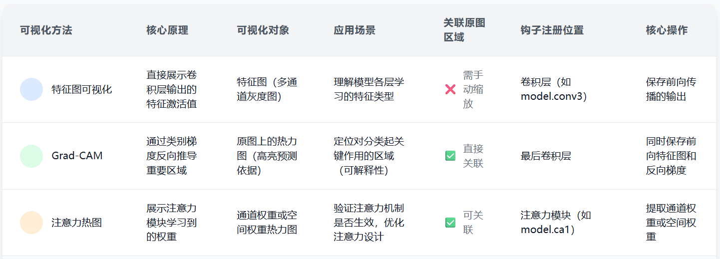
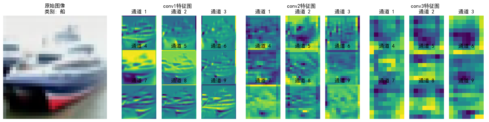
不同CNN层的特征图：不同通道的特征图
什么是注意力：注意力家族，类似于动物园，都是不同的模块，好不好试了才知道。
通道注意力：模型的定义和插入的位置
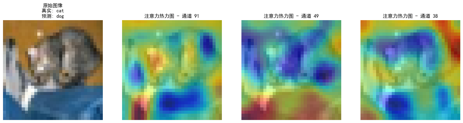
通道注意力后的特征图和热力图

内容参考

作业：

今日代码较多，理解逻辑即可
对比不同卷积层特征图可视化的结果（可选）

一、CNN特征图可视化实现

复制代码

import torch
import matplotlib.pyplot as plt

def visualize_feature_maps(model, input_tensor):
    # 注册钩子获取中间层输出
    features = []
    def hook(module, input, output):
        features.append(output.detach().cpu())
    
    # 选择不同卷积层观察
    target_layers = [
        model.layer1[0].conv1,
        model.layer2[0].conv1,
        model.layer3[0].conv1
    ]
    
    handles = []
    for layer in target_layers:
        handles.append(layer.register_forward_hook(hook))
    
    # 前向传播
    with torch.no_grad():
        _ = model(input_tensor.unsqueeze(0))
    
    # 移除钩子
    for handle in handles:
        handle.remove()
    
    # 可视化不同层特征图
    fig, axes = plt.subplots(len(target_layers), 5, figsize=(20, 10))
    for i, feat in enumerate(features):
        for j in range(5):  # 显示前5个通道
            axes[i,j].imshow(feat[0, j].numpy(), cmap='viridis')
            axes[i,j].axis('off')
    plt.show()

二、通道注意力模块示例

复制代码

class ChannelAttention(nn.Module):
    def __init__(self, in_channels, reduction=16):
        super().__init__()
        self.avg_pool = nn.AdaptiveAvgPool2d(1)
        self.max_pool = nn.AdaptiveMaxPool2d(1)
        
        self.fc = nn.Sequential(
            nn.Linear(in_channels, in_channels // reduction),
            nn.ReLU(),
            nn.Linear(in_channels // reduction, in_channels),
            nn.Sigmoid()
        )
    
    def forward(self, x):
        # ... existing code ...
        return x * attention_weights  # 应用注意力权重

三、热力图生成方法

复制代码

def generate_heatmap(model, input_img):
    # 前向传播获取梯度
    model.eval()
    input_img.requires_grad = True
    output = model(input_img)
    pred_class = output.argmax(dim=1).item()
    
    # 反向传播计算梯度
    model.zero_grad()
    output[0, pred_class].backward()
    
    # 获取最后一个卷积层的梯度
    gradients = model.layer4[1].conv2.weight.grad
    pooled_gradients = torch.mean(gradients, dim=[0,2,3])
    
    # 生成热力图
    activations = model.layer4[1].conv2.activations.detach()
    for i in range(activations.shape[1]):
        activations[:,i,:,:] *= pooled_gradients[i]
    heatmap = torch.mean(activations, dim=1).squeeze()
    
    return heatmap