pytorch入门：利用pytorch进行线性预测

进行深度学习主要分为四步，首先准备数据，然后定义模型，再定义损失值和优化器，最后进行模型的训练，当然训练后可以用模型来进行预测；

这里先使用一个最简单的模型来进行入门，即使用pytorch来进行一个线性模型的预测，利用线性模型可以用来进行一些简单的预测，虽然这些预测使用机器学习也能胜任；

（1）准备数据

首先是产生数据集，这里使用一个线性函数，在函数中添加一些随机正态噪声，在创建数据集时候，我们顺便留下一些x数据用来后面进行预测，因为我们的y数据是加入噪声的数据，因此后面预测对比的是直接使用函数生成的y的数据

python 复制代码

def creat_linear_data():
    x = np.array([[float(np.random.randn(1))] for i in range(100)])
    y = np.array([[10 * x[i][0] + float(np.random.randn(1)) + 3] for i in range(100)])
    x_train, x_test, y_train, y_test = train_test_split(x, y, test_size=0.2)
    # print(x, y)
    return x_train, x_test, y_train, y_test

另外调用此函数获得的是array类型的数据，要使用pytorch进行模型训练，需要我们将数据转换为tensor类型的数据

python 复制代码

x_train, x_test, y_train, y_test = creat_linear_data()
x_data, x_test = torch.tensor(x_train, dtype=torch.float32), torch.tensor(x_test, dtype=torch.float32)
y_data, y_test = torch.tensor(y_train, dtype=torch.float32), torch.tensor(y_test, dtype=torch.float32)

（2）定义模型

由于我们只使用了简单的线性模型，因此定义模型很简单，只要定义一个线性的网络结构即可，定义前向传播函数也只是进行了一层传递；

另外要注意的是在定义线性网络类时，记得要继承父类nn.Module

python 复制代码

class linear_net(nn.Module):
    def __init__(self):
        super(linear_net, self).__init__()    # 继承父类初始化

        self.linear1 = nn.Linear(1, 1)  # 第一个参数为输入数据维度，第二个参数为输出数据维度

    def forward(self, x):

        y = self.linear1(x) # 前向传播
        return y

（3）定义损失函数和优化器

损失函数可以根据训练模型的不同选择不同的损失函数，这里由于模型是自己生成的，因此可以选择均方误差作为损失函数，这里的优化器选择随机梯度下降SGD，也可以选择其他优化器

另外在这一步中可以顺便进行模型的初始化

python 复制代码

model = linear_net()
criterion = nn.MSELoss(size_average=False)    # 损失函数
optimizer = optim.SGD(model.parameters(), lr=0.01)   # 优化器

（4）训练

进行完前面的步骤后就可以利用数据对模型进行训练了，模型训练分为三步，第一步是进行前馈，也就是计算训练中的猜测值，通过猜测值和真实值计算损失函数，第二步是进行反馈，通过损失计算梯度，第三部是进行更新，使用优化器来对权重进行更新以减少损失

python 复制代码

loss_list = [0.0 for i in range(50)]

for i in range(50):
    y_pre = model(x_data)   # 前向传播
    loss = criterion(y_pre, y_data) # 计算损失
    # print(i, loss.item())
    loss_list[i] = loss.item()  # 存储损失
    optimizer.zero_grad()   # 清空梯度
    loss.backward() # 反向传播
    optimizer.step()    # 更新参数

要注意的是，在每次训练后我们都要进行手动清空梯度，因为pytorch默认为累计梯度，如果不进行手动清空，会导致梯度累计越来越大，进而导致参数更新过大，模型无法收敛

（5）预测

进行完训练后我们可以进行模型的保存，也可以利用模型来进行推理，这里使用数据是之前生成数据时分割的测试数据，对比数据使用函数来进行生成，使用matplotlib进行绘图对比，顺便把损失值也进行绘制

python 复制代码

model.eval()    # 测试
with torch.no_grad():   # 测试时关闭梯度
    y_pre = model(torch.tensor(x_test, dtype=torch.float32))
    print(f"W:{model.linear1.weight.item()}")
    print(f"b:{model.linear1.bias.item()}")

fig, axs = plt.subplots(1, 2)
axs[0].plot(loss_list)
axs[1].scatter(x_test, y_pre, c='r')
axs[1].scatter(x_test, 10*x_test + 3, c='b')

plt.show()

最终图显示训练过程中的损失值和利用不同颜色的预测值和真实值

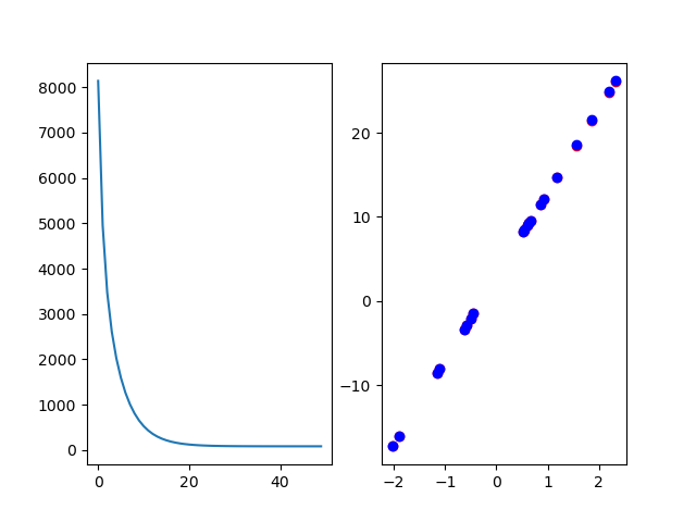
可以看到损失函数在进行到20左右时候不再变化，说明此时模型已经收敛；同时可以看到预测值和真实值几乎完全覆盖，由于数据比较简单，因此训练起来也比较简单；

可以打印参数进行对比

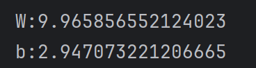
和我们设置w=10以及b=3十分接近，证明这个训练还是比较成功的

（6）整体代码

python 复制代码

class linear_net(nn.Module):
    def __init__(self):
        super(linear_net, self).__init__()    # 继承父类初始化

        self.linear1 = nn.Linear(1, 1)  # 第一个参数为输入数据维度，第二个参数为输出数据维度

    def forward(self, x):

        y = self.linear1(x) # 前向传播
        return y

def creat_linear_data():
    x = np.array([[float(np.random.randn(1))] for i in range(100)])
    y = np.array([[10 * x[i][0] + float(np.random.randn(1)) + 3] for i in range(100)])
    x_train, x_test, y_train, y_test = train_test_split(x, y, test_size=0.2)
    # print(x, y)
    return x_train, x_test, y_train, y_test

x_train, x_test, y_train, y_test = creat_linear_data()
x_data, x_test = torch.tensor(x_train, dtype=torch.float32), torch.tensor(x_test, dtype=torch.float32)
y_data, y_test = torch.tensor(y_train, dtype=torch.float32), torch.tensor(y_test, dtype=torch.float32)

model = linear_net()
criterion = nn.MSELoss(size_average=False)    # 损失函数
optimizer = optim.SGD(model.parameters(), lr=0.01)   # 优化器


loss_list = [0.0 for i in range(50)]

for i in range(50):
    y_pre = model(x_data)   # 前向传播
    loss = criterion(y_pre, y_data) # 计算损失
    # print(i, loss.item())
    loss_list[i] = loss.item()  # 存储损失
    optimizer.zero_grad()   # 清空梯度
    loss.backward() # 反向传播
    optimizer.step()    # 更新参数

model.eval()    # 测试
with torch.no_grad():   # 测试时关闭梯度
    y_pre = model(torch.tensor(x_test, dtype=torch.float32))
    print(f"W:{model.linear1.weight.item()}")
    print(f"b:{model.linear1.bias.item()}")

fig, axs = plt.subplots(1, 2)
axs[0].plot(loss_list)
axs[1].scatter(x_test, y_pre, c='r')
axs[1].scatter(x_test, 10*x_test + 3, c='b')

plt.show()