一、说明
在本文中,我们将通过简单的类比、清晰的解释和动手示例来揭开特征向量和特征值背后的神秘面纱。让我们一起探讨为什么这些概念在简化复杂数据和发现隐藏的见解方面如此重要。
二、直观解释
2.1 特征向量到底是什么?
想象一下,试着推开一扇旋转门。如果你径直向前推,门会毫不费力地打开。然而,如果向侧面或对角线方向推,你就不会有太大的进展。同样,在矩阵和变换的数学世界中,特定的特殊方向使得变换变得非常简单。
这些特殊的方向被称为特征向量,它们之所以独特,是因为当你应用变换(用矩阵表示)时,这些向量会保持指向其原始方向。它们不会旋转或扭曲;相反,它们只是拉伸或收缩。特征向量拉伸或收缩的倍数就是其对应的特征值。
从数学上来说,我们简单地表达这种关系:
Av=λvAv=\lambda vAv=λv
在这里:
A 是表示变换的方阵。
v 是特征向量(特殊的非零向量)。
λ (lambda)是特征值,即沿该方向拉伸或收缩的量。
特征向量背后的几何直觉
A对大多数向量v采取变换,v既有方向变化(旋转),和长度变化(伸缩),特征向量在矩阵变换下的行为类似:它们的方向保持不变。它们可能会被拉伸或挤压在一起,但它们永远不会偏离轨道或改变方向。
2.2 从反问题进行考虑
我们首先考察,能否对于任意向量(非零),找到一个变换矩阵A,使的A对v变换不改变v的方向。
v=λ(cosθsinθ)v =\lambda \begin{pmatrix} cos\theta \\ sin\theta \end{pmatrix}v=λ(cosθsinθ)
给出一个A如下:
A=(mabn)A = \begin{pmatrix} m & a \\ b & n \end{pmatrix}A=(mban)
带入Av=λvAv=\lambda vAv=λv
得到:
a=(λ−m)cosθsinθ a = \frac{(\lambda - m)cos\theta}{sin\theta}a=sinθ(λ−m)cosθ
b=(λ−n)sinθcosθ b = \frac{(\lambda - n)sin\theta}{cos\theta}b=cosθ(λ−n)sinθ
所以:v=λ(cosθsinθ)v =\lambda \begin{pmatrix} cos\theta \\ sin\theta \end{pmatrix}v=λ(cosθsinθ)
向量v的特征矩阵是:
A=(m(λ−m)cosθsinθ(λ−n)sinθcosθn)A = \begin{pmatrix} m & \frac{(\lambda - m)cos\theta}{sin\theta} \\ \frac{(\lambda - n)sin\theta}{cos\theta} & n \end{pmatrix}A=(mcosθ(λ−n)sinθsinθ(λ−m)cosθn)
以上说明一个事实,对于任意一个非零向量v,我们可以给出对角线上的任意值m和n,便可以构造v的特征矩阵,显然
1)特征矩阵的数量是无穷无尽的。
2)特征矩阵和向量v存在某种制约关系。
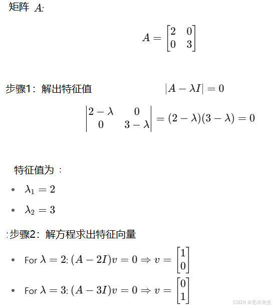
2.3 正面问题叙事
所谓正面问题,就是给出一个矩阵,求它对应的特征向量。
任意给出矩阵,求出特征向量的代码
import matplotlib.pyplot as plt
import numpy as np

# Define the matrix A
A = np.array([[2, 0], [0, 3]])

# Define a set of original vectors
original_vectors = np.array([
    [1, 0],  # eigenvector for lambda=2
    [0, 1],  # eigenvector for lambda=3
    [1, 1],  # not an eigenvector
    [1, -1]  # not an eigenvector
])

# Apply transformation
transformed_vectors = original_vectors @ A.T

# Plot
fig, ax = plt.subplots(figsize=(8, 8))
colors = ['blue', 'green', 'gray', 'gray']
labels = ['v1 (λ=2)', 'v2 (λ=3)', 'non-eigen', 'non-eigen']

# Draw original and transformed vectors
for i, vec in enumerate(original_vectors):
    # Original vector
    ax.quiver(0, 0, vec[0], vec[1], angles='xy', scale_units='xy', scale=1, color=colors[i],
              label=f'{labels[i]} (original)', alpha=0.5)
    # Transformed vector
    t_vec = transformed_vectors[i]
    ax.quiver(0, 0, t_vec[0], t_vec[1], angles='xy', scale_units='xy', scale=1, color=colors[i],
              alpha=1.0, linestyle='solid', label=f'{labels[i]} (transformed)')

# Settings
ax.set_xlim(-4, 4)
ax.set_ylim(-4, 4)
ax.axhline(0, color='black', lw=1)
ax.axvline(0, color='black', lw=1)
ax.set_aspect('equal')
ax.set_title('Matrix A = [[2, 0], [0, 3]] acting on vectors')
ax.legend(loc='upper left')
plt.grid(True)
plt.show()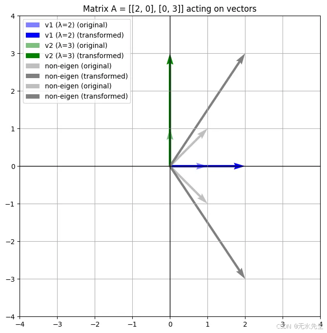
2.3 更一般的现象
以下是更新后的剧本:
蓝色和绿色向量表示矩阵 AAA 的特征向量,它们经过缩放(未旋转)。
灰色向量表示在变换下发生变化的方向,表明它们不是特征向量。
变换后的向量被叠加起来以显示矩阵如何缩放每个向量。

与之前的对角矩阵不同,这个矩阵混合了 x 和 y 分量。尽管如此,特征向量仍然揭示了矩阵表现为简单缩放的方向。
import matplotlib.pyplot as plt
import numpy as np

# Define matrix A
A = np.array([[4, 2], [1, 3]])

# Define original vectors including eigenvectors and some extras
original_vectors = np.array([
    [2, 1],    # eigenvector for lambda=5
    [-1, 1],   # eigenvector for lambda=2
    [1, 0],    # test vector
    [0, 1],    # test vector
])

# Apply transformation
transformed_vectors = original_vectors @ A.T

# Plot
fig, ax = plt.subplots(figsize=(8, 8))
colors = ['blue', 'green', 'gray', 'gray']
labels = ['v1 (λ=5)', 'v2 (λ=2)', 'test x-axis', 'test y-axis']

# Draw original and transformed vectors
for i, vec in enumerate(original_vectors):
    ax.quiver(0, 0, vec[0], vec[1], angles='xy', scale_units='xy', scale=1,
              color=colors[i], label=f'{labels[i]} (original)', alpha=0.5)
    t_vec = transformed_vectors[i]
    ax.quiver(0, 0, t_vec[0], t_vec[1], angles='xy', scale_units='xy', scale=1,
              color=colors[i], label=f'{labels[i]} (transformed)', linestyle='-')

# Settings
ax.set_xlim(-8, 8)
ax.set_ylim(-8, 8)
ax.axhline(0, color='black', lw=1)
ax.axvline(0, color='black', lw=1)
ax.set_aspect('equal')
ax.set_title('Matrix A = [[4, 2], [1, 3]] acting on various vectors')
ax.legend(loc='upper left')
plt.grid(True)
plt.show()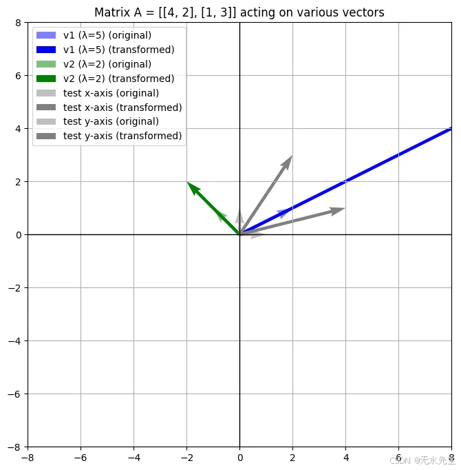
三、机器学习如何使用特征向量的?
3.1 为什么特征向量和特征值在机器学习中很重要
假设你是一位数据科学家,走进一艘宇宙飞船(也就是你的数据集)里一间凌乱的控制室。所有东西都闪烁着、嗡嗡作响,令人眼花缭乱------每行都有数百个特征。你问道:
"我应该关注哪些主要控制点?信号最强的地方在哪里?"
3.2 高维问题
在现实世界的数据集中,我们经常处理高维数据------每个数据点有数百或数千个特征(列)。例如:
大小为 28×28 的灰度图像具有 784 个像素 = 784 个特征。
一个文本文档可能有数千个词嵌入。
传感器读数或时间序列数据的维度可能非常大。
但更多特征并不总是意味着更多信息。许多维度通常:
冗余(多个特征传达相似的模式)
低方差(它们在数据点之间几乎不会发生变化)
嘈杂(它们增加了混乱,而不是清晰度)
这时,特征值和特征向量就成了我们的数学放大镜。它们帮助我们回答:
数据变化最大的方向是什么?
哪些功能真正具有信息量?
我们可以在不丢失关键信息的情况下降低维度吗?
3.2 应用1:基本笔触
想象一下艺术家细致的肖像画。从远处看,几笔粗犷的笔触便能讲述整个故事。复杂的笔触纹理?它们固然好看,但并非必需。
带有特征向量的 SVD 有助于我们保留粗体笔触(主要图案),并忽略精细纹理(次要特征值)。让我们使用 SVD 压缩一张灰度图像。
加载图像并转换为灰度。
应用 SVD 来获取特征分量。
仅使用前 k 个组件重建图像。
import numpy as np
import matplotlib.pyplot as plt
from skimage import data, color
from skimage.transform import resize


# Load a real image (camera photo) and resize for speed
image = color.rgb2gray(data.coffee())  # Load grayscale version
image = resize(image, (128, 128), anti_aliasing=True)

# Step 1: Apply SVD
U, S, VT = np.linalg.svd(image, full_matrices=False)

# Step 2: Reconstruct using top-k eigen-components
def compress_image(k):
    compressed = (U[:, :k] @ np.diag(S[:k]) @ VT[:k, :])
    return compressed

# Step 3: Show original and compressed images
ks = [5,10,15, 20, 50, 100]
plt.figure(figsize=(10, 6))
for i, k in enumerate(ks):
    plt.subplot(1, len(ks), i + 1)
    plt.imshow(compress_image(k), cmap='gray')
    plt.title(f'{k} components')
    plt.axis('off')
plt.suptitle('Image Compression Using SVD (Eigen Decomposition)')
plt.show()
3.3 应用2:在一堆书中寻找核心含义:
想象一下,你拿到一百本外语书,你的目标是理解其中的主题。你注意到,尽管书页繁多,但一些重复的词语模式却主导着信息。如果你能识别出这些核心思想,就不需要逐字逐句地阅读了。
特征向量的作用就是:找到数据集中变异的核心轴。特征值则告诉你每个轴包含多少信息(方差)。结果呢?你只需要保留关键方向,忽略其他方向。
from sklearn.datasets import fetch_20newsgroups
from sklearn.feature_extraction.text import TfidfVectorizer
from sklearn.decomposition import TruncatedSVD,PCA
import matplotlib.pyplot as plt

# Load a subset of newsgroup articles
newsgroups = fetch_20newsgroups(subset='train', categories=['sci.space', 'rec.sport.baseball', 'comp.graphics'], remove=('headers', 'footers', 'quotes'))

# Convert text to TF-IDF feature matrix
vectorizer = TfidfVectorizer(stop_words='english', max_features=1000)
X = vectorizer.fit_transform(newsgroups.data)

# Apply SVD (LSA) to reduce dimensionality
lsa = PCA(n_components=2)
X_lsa = lsa.fit_transform(X)

# Plot the documents in 2D LSA space
plt.scatter(X_lsa[:, 0], X_lsa[:, 1], c=newsgroups.target, cmap='tab10', alpha=0.6)
plt.title('20 Newsgroups Text Data in 2D LSA Space')
plt.xlabel('Component 1')
plt.ylabel('Component 2')
plt.colorbar()
plt.show()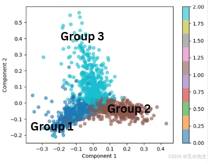
在这个例子中,特征向量表示文档中的主要主题。特征值告诉我们每个主题捕获了多少方差(信息)。结果就像在海量文本库中放大到信息量最大的主题。
3.4 应用3:网页排名(PageRank)
让我们把互联网想象成一张巨大的蜘蛛网,每个网页都是一个节点,每个超链接都是连接各个页面的线索。被许多重要页面链接的页面本身就应该被视为重要页面。
我们如何从数学上确定哪个页面最"重要"?
通过计算链接矩阵的特征向量!
import numpy as np
import matplotlib.pyplot as plt
import networkx as nx

# Define the link matrix L
L = np.array([
    [0, 1, 1, 0],  # A receives from B and C
    [0, 0, 0, 1],  # B receives from D
    [1, 0, 0, 1],  # C receives from A and D
    [0, 0, 1, 0],  # D receives from C
], dtype=float)

# Normalize columns to create the transition probability matrix
P = L / L.sum(axis=0, keepdims=True)

# Damping factor and Google matrix
alpha = 0.85
n = P.shape[0]
G = alpha * P + (1 - alpha) / n * np.ones((n, n))

# Eigen decomposition
eigvals, eigvecs = np.linalg.eig(G)

# Get the principal eigenvector (corresponding to eigenvalue ~1)
principal_eigvec = np.abs(eigvecs[:, np.isclose(eigvals, 1)])
pagerank = principal_eigvec / principal_eigvec.sum()

# Graph visualization
labels = ['A', 'B', 'C', 'D']
edges = [(1, 0), (2, 0), (3, 1), (0, 2), (3, 2), (2, 3)]
G_nx = nx.DiGraph()
G_nx.add_edges_from(edges)

# Position nodes in a circle
pos = nx.circular_layout(G_nx)

# Draw the graph
plt.figure(figsize=(8, 6))
node_size = 3000 * pagerank.flatten()
nx.draw_networkx(G_nx, pos, with_labels=True, labels=dict(zip(range(n), labels)),
                 node_color='lightblue', node_size=node_size, edge_color='gray', arrows=True)
plt.title("Simple Web Graph --- Node Size Reflects PageRank")
plt.axis('off')
plt.show()

pagerank.flatten()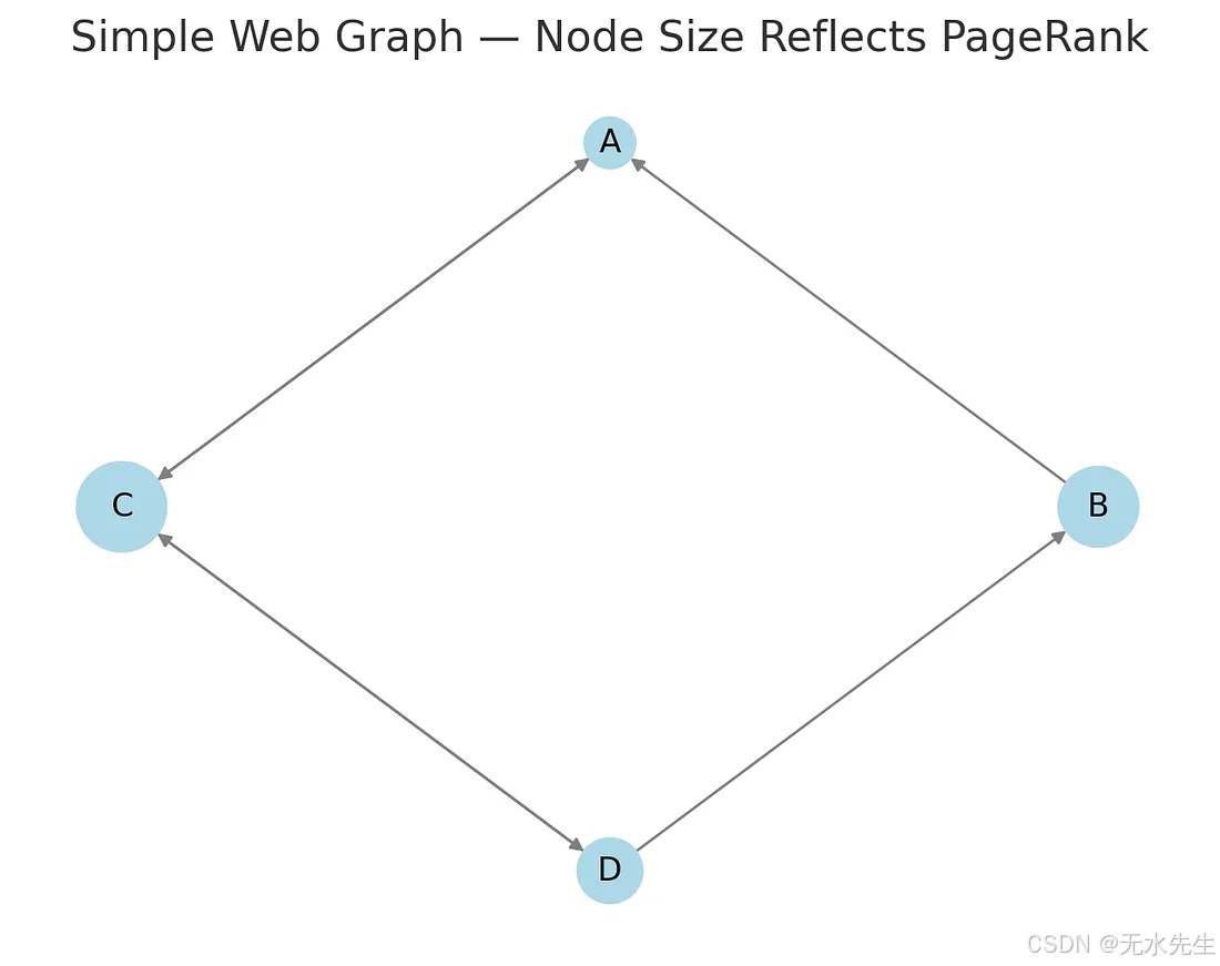
每个节点(A、B、C、D)代表一个网页。
定向箭头表示页面之间的链接。
节点大小反映了 PageRank:每个页面的重要性。
结果:
页面 C具有最高的 PageRank(≈ 0.378),重要页面大量链接到该页面。
接下来是页面 A(≈ 0.302)------连接性也很好。
页面 D(≈ 0.198)和页面 B(≈ 0.122)在网络中不太中心。
通过计算修改后的转移矩阵的特征值~1 对应的特征向量,我们捕获了网页之间重要性的稳态分布,这是 Google 原始 PageRank 的核心。
此外,PageRank 还可以用于识别有影响力的用户。在这种情况下,使用 PageRank 算法有助于识别网络中最受信任的用户。该算法根据传入边的结构为每个节点分配一个分数,从而有效地突出显示有影响力的用户。
import networkx as nx
import matplotlib.pyplot as plt
# download the dataset from
#https://snap.stanford.edu/data/soc-Epinions1.html
# e.g or input
# FromNodeId ToNodeId
# 0 4
# 0 5
# 0 7

# Read the soc-Epinions1.txt file and load edges
file_path = "soc-Epinions1.txt"

# Skip lines that start with '#' and read edges
edges = []
with open(file_path, 'r') as f:
    for line in f:
        if not line.startswith("#"):
            from_node, to_node = map(int, line.strip().split())
            edges.append((from_node, to_node))

# Build directed graph
G = nx.DiGraph()
G.add_edges_from(edges)

# Compute PageRank, based on Eigenvalue and Eigen vectors
# The principal eigenvector (the eigenvector associated with the largest eigenvalue) provides the PageRank scores.
pagerank_scores = nx.pagerank(G, alpha=0.85)

# Display top 10 PageRank scores
top_users = sorted(pagerank_scores.items(), key=lambda x: -x[1])[:10]
for user, score in top_users:
    print(f"User {user}: {score:.6f}")

# Visualize subgraph of top 10 users
top_nodes = [user for user, _ in top_users]
subgraph = G.subgraph(top_nodes)

plt.figure(figsize=(10, 7))
pos = nx.spring_layout(subgraph, seed=42)
node_sizes = [10000 * pagerank_scores[node] for node in subgraph.nodes()]
nx.draw_networkx_nodes(subgraph, pos, node_size=node_sizes, node_color='lightgreen')
nx.draw_networkx_edges(subgraph, pos, arrowstyle='->', arrowsize=15, edge_color='gray')
nx.draw_networkx_labels(subgraph, pos, font_size=10)
plt.title("Top 10 Influential Users in Epinions Network (PageRank)")
plt.axis('off')
plt.show()
###output###
User 18: 0.004657
User 737: 0.002881
User 1719: 0.002155
User 790: 0.002122
User 118: 0.002059
User 136: 0.002035
User 143: 0.002004
User 40: 0.001592
User 1619: 0.001526
User 4415: 0.001478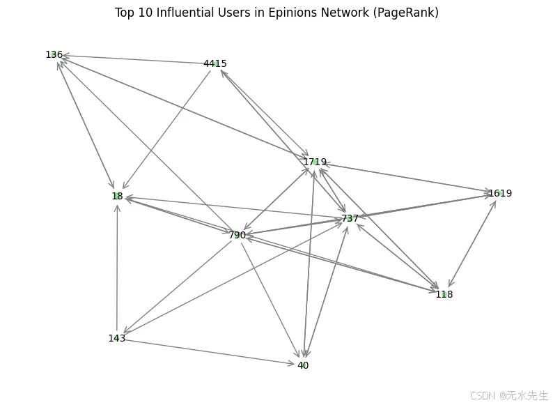
四、与其它问题的关系
在这些例子中,我提到了PCA、SVD和特征向量。它们之间有什么关系?
4.1 主成分分析(PCA)
一种降低数据维数的统计方法。PCA 可以简化数据,同时尽可能多地保留方差(信息)。
与特征向量/值的联系:
PCA 使用数据协方差矩阵的特征向量。
特征向量代表最大方差的方向("主成分")。
特征值表示每个特征向量捕获的方差量。
PCA的工作原理:
计算数据的协方差矩阵。
找到它的特征向量和特征值。
保留前k 个特征向量(最大特征值),将数据投影到这些新轴上以降低维数。
4.2 奇异值分解(SVD)
将任何矩形矩阵分解为三个更简单的矩阵的方法。
对于任何矩阵 A:
A=U×Σ×VTA=U×Σ×V^TA=U×Σ×VT
U 和 V:正交矩阵(表示旋转/反射)。
Σ(Sigma):对角矩阵(奇异值,表示缩放)。
与特征向量/值和PCA的连接:
SVD 将特征分解推广到任何矩阵,甚至非方阵。
SVD 与 PCA 的关系:
PCA 是专门应用于协方差矩阵的SVD 。
PCA 使用特征分解(一种特殊情况),而 SVD 可以分解任何矩阵。
将显示缩放图像
五、结论
- 矩阵的作用类似于可以旋转、拉伸或剪切空间的变换。将它们可视化为网格扭曲机是建立直觉的好方法。
- 特征向量是变换不会旋转的特殊方向。沿这些方向的向量只会被变换缩放(或翻转),保持在同一直线上。
- 特征值是特征向量缩放的因子。它告诉我们变换是拉伸、收缩还是翻转特征向量线上的向量。
通过关注特征向量和特征值,我们常常可以简化复杂的问题。它们有助于矩阵对角化,简化计算,并揭示变换的基本性质(例如守恒定律、拉伸主轴等)。但在几何层面上,你可以更清晰地理解和把握。