机器学习 - Kaggle项目实践（8）Spooky Author Identification 作者识别

Spooky Author Identification | Kaggle

Approaching (Almost) Any NLP Problem on Kaggle （参考）

Spooky Author Identification | Kaggle （My work）

根据三位的一些作品训练集，三分类测试集是哪个作家写的概率。

目录

[1. 数据导入&格式display](#1. 数据导入&格式display)

[2. 损失函数的定义](#2. 损失函数的定义)

[3. 数据准备](#3. 数据准备)

[4. 两种向量化编码 TF-IDF和词频统计Count](#4. 两种向量化编码 TF-IDF和词频统计Count)

[5. 机器学习分类模型](#5. 机器学习分类模型)

[5.1 逻辑回归](#5.1 逻辑回归)

[5.2 朴素贝叶斯模型](#5.2 朴素贝叶斯模型)

[5.3 对TF-IDF SVD降维+标准化后 SVM](#5.3 对TF-IDF SVD降维+标准化后 SVM)

[6. Grid_Search 参数调优](#6. Grid_Search 参数调优)

[6.1 Grid_Search_SVM](#6.1 Grid_Search_SVM)

[6.2 Grid_Search_贝叶斯](#6.2 Grid_Search_贝叶斯)

[7. GloVe词向量 + XGboost](#7. GloVe词向量 + XGboost)

[8. GloVe词向量 + 深度学习](#8. GloVe词向量 + 深度学习)

[8.1 构建embedding_matrix 作为词嵌入层](#8.1 构建embedding_matrix 作为词嵌入层)

[8.2 LSTM / 双头LSTM / GRU](#8.2 LSTM / 双头LSTM / GRU)

[8.3 预测+提交](#8.3 预测+提交)

---

1. 数据导入&格式display

import pandas as pd
import numpy as np
train = pd.read_csv('/kaggle/input/spooky-author-identification/train.zip')
test = pd.read_csv('/kaggle/input/spooky-author-identification/test.zip')
sample = pd.read_csv('/kaggle/input/spooky-author-identification/sample_submission.zip')

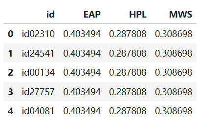
display(train.head())
display(test.head())
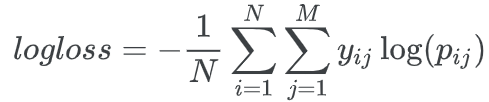
display(sample.head())

test 数据包含id 和 text内容；train中还多一个标签 哪个作者写的。

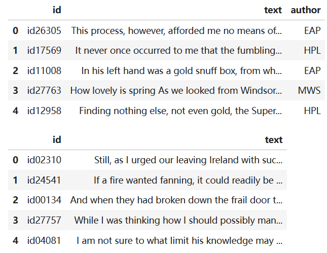
submission_sample中为 id 以及text为每个作者的概率（每行均为训练集中每个作者的比例）

2. 损失函数的定义

多类别对数损失函数；仅i属于类别j时 y=1；即 pij 越大越好

def multiclass_logloss(actual, predicted, eps=1e-15):
    # 步骤1: 将整数标签转换为one-hot编码
    if len(actual.shape) == 1:
        actual2 = np.zeros((actual.shape[0], predicted.shape[1]))
        for i, val in enumerate(actual):
            actual2[i, val] = 1  # 对应 y_ij = 1 (当j=真实类别时)
        actual = actual2

    # 步骤2: 防止log(0)的情况，将概率裁剪到[eps, 1-eps]范围
    clip = np.clip(predicted, eps, 1 - eps)  # 对应 p_ij
    
    # 步骤3: 计算损失
    rows = actual.shape[0]  # 对应 N (样本数量)
    vsota = np.sum(actual * np.log(clip))  # 对应 ΣΣ [y_ij * log(p_ij)]
    
    # 步骤4: 最终计算
    return -1.0 / rows * vsota  # 对应 - (1/N) * ΣΣ [y_ij * log(p_ij)]

3. 数据准备

target为作者名称 使用LabelEncoder() 转换为0 1 2 编码； 并划分训练集测试集

from sklearn import preprocessing
from sklearn.model_selection import train_test_split
lbl_enc = preprocessing.LabelEncoder()
y = lbl_enc.fit_transform(train.author.values)
xtrain, xvalid, ytrain, yvalid = train_test_split(train.text.values, y, 
                                                  stratify=y, 
                                                  random_state=42, 
                                                  test_size=0.1, shuffle=True)

4. 两种向量化编码 TF-IDF和词频统计Count

from sklearn.feature_extraction.text import TfidfVectorizer, CountVectorizer

# TF-IDF特征提取
tfv = TfidfVectorizer(min_df=3, max_features=None, 
            strip_accents='unicode', analyzer='word', token_pattern=r'\w{1,}',
            ngram_range=(1, 3), use_idf=1, smooth_idf=1, sublinear_tf=1,
            stop_words='english')

# 拟合并转换数据
tfv.fit(list(xtrain) + list(xvalid))  # 在训练集+验证集上学习词汇表
xtrain_tfv = tfv.transform(xtrain)    # 转换训练集为TF-IDF矩阵
xvalid_tfv = tfv.transform(xvalid)    # 转换验证集为TF-IDF矩阵

# Count向量化特征提取
ctv = CountVectorizer(
    analyzer='word',            # 按单词进行分词
    token_pattern=r'\w{1,}',    # 匹配至少1个字符的单词
    ngram_range=(1, 3),         # 使用1-gram, 2-gram, 3-gram
    stop_words='english'        # 移除英文停用词
)

# 拟合并转换数据
ctv.fit(list(xtrain) + list(xvalid))  # 在训练集+验证集上学习词汇表
xtrain_ctv = ctv.transform(xtrain)    # 转换训练集为词频矩阵
xvalid_ctv = ctv.transform(xvalid)    # 转换验证集为词频矩阵

print(f"TF-IDF特征维度: {xtrain_tfv.shape}")
print(f"Count特征维度: {xtrain_ctv.shape}")

5. 机器学习分类模型

5.1 逻辑回归

fit + 预测 predict_proba + 之前定义的损失

from sklearn.linear_model import LogisticRegression
# Fitting a simple Logistic Regression on TFIDF
clf = LogisticRegression(C=1.0)
clf.fit(xtrain_tfv, ytrain)
predictions = clf.predict_proba(xvalid_tfv)

print ("logloss: %0.3f " % multiclass_logloss(yvalid, predictions))

# Fitting a simple Logistic Regression on Counts
clf = LogisticRegression(C=1.0)
clf.fit(xtrain_ctv, ytrain)
predictions = clf.predict_proba(xvalid_ctv)

print ("logloss: %0.3f " % multiclass_logloss(yvalid, predictions))

5.2 朴素贝叶斯模型

from sklearn.naive_bayes import MultinomialNB
# Fitting a simple Naive Bayes on TFIDF
clf = MultinomialNB()
clf.fit(xtrain_tfv, ytrain)
predictions = clf.predict_proba(xvalid_tfv)

print ("logloss: %0.3f " % multiclass_logloss(yvalid, predictions))

# Fitting a simple Naive Bayes on Counts
clf = MultinomialNB()
clf.fit(xtrain_ctv, ytrain)
predictions = clf.predict_proba(xvalid_ctv)

print ("logloss: %0.3f " % multiclass_logloss(yvalid, predictions))

5.3 对TF-IDF SVD降维+标准化后 SVM

因为SVM对特征尺度敏感 需要降维+scale 加快收敛

from sklearn import decomposition,preprocessing
from sklearn.svm import SVC

# 1. SVD降维
svd = decomposition.TruncatedSVD(n_components=120)
svd.fit(xtrain_tfv)
xtrain_svd = svd.transform(xtrain_tfv)
xvalid_svd = svd.transform(xvalid_tfv)

# 2. 数据标准化
scl = preprocessing.StandardScaler()
scl.fit(xtrain_svd)
xtrain_svd_scl = scl.transform(xtrain_svd)
xvalid_svd_scl = scl.transform(xvalid_svd)

# 3. SVM训练和评估
clf = SVC(C=1.0, probability=True, random_state=42)
clf.fit(xtrain_svd_scl, ytrain)
predictions = clf.predict_proba(xvalid_svd_scl)

print("SVM在SVD降维特征上的logloss: %0.3f" % multiclass_logloss(yvalid, predictions))

6. Grid_Search 参数调优

需要准备 1.estimator模型管道 2.param_grid参数网络 3.scoring评分器

6.1 Grid_Search_SVM

1. 根据损失函数 创建评分器

from sklearn import metrics, pipeline
from sklearn.model_selection import GridSearchCV
# 1. 创建评分器
mll_scorer = metrics.make_scorer(multiclass_logloss, greater_is_better=False, needs_proba=True)
# 自定义的多类别对数损失函数转换为scikit-learn的评分器
# greater_is_better=False：logloss越小越好，所以设为False
# needs_proba=True：需要概率预测而不是类别标签

2. 降维+标准化+SVM 三个步骤创建管道

# 2. 创建管道 三个步骤
svd = decomposition.TruncatedSVD()
scl = preprocessing.StandardScaler()
lr_model = LogisticRegression()

clf = pipeline.Pipeline([
    ('svd', svd),      # 第一步：SVD降维
    ('scl', scl),      # 第二步：数据标准化
    ('lr', lr_model)   # 第三步：逻辑回归
])

3. 参数网络 降维数 / 正则化 类型与大小

# 3. 定义参数网格
param_grid = {
    'svd__n_components': [120, 180],  # SVD组件数
    'lr__C': [0.1, 1.0, 10],         # 正则化强度
    'lr__penalty': ['l1', 'l2']      # 正则化类型
}

4. 执行网格搜索 输出最优结果

# 4. 网格搜索
model = GridSearchCV(estimator=clf, param_grid=param_grid, scoring=mll_scorer,
                                 verbose=10, n_jobs=-1, refit=True, cv=2)

# 5. 执行网格搜索
model.fit(xtrain_tfv, ytrain)

# 6. 输出最佳结果
print("Best score: %0.3f" % model.best_score_)
print("Best parameters set:")
best_parameters = model.best_estimator_.get_params()
for param_name in sorted(param_grid.keys()):
    print("\t%s: %r" % (param_name, best_parameters[param_name]))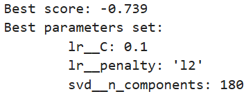

6.2 Grid_Search_贝叶斯

参数：拉普拉斯平滑（Laplace smoothing） 的强度

# GridSearch 三个准备
nb_model = MultinomialNB()

clf = pipeline.Pipeline([('nb', nb_model)])

param_grid = {'nb__alpha': [0.001, 0.01, 0.1, 1, 10, 100]}

model = GridSearchCV(estimator=clf, param_grid=param_grid, scoring=mll_scorer,
                                 verbose=10, n_jobs=-1, refit=True, cv=2)
# 搜索输出最佳结果
model.fit(xtrain_tfv, ytrain)
print("Best score: %0.3f" % model.best_score_)
print("Best parameters set:")
best_parameters = model.best_estimator_.get_params()
for param_name in sorted(param_grid.keys()):
    print("\t%s: %r" % (param_name, best_parameters[param_name]))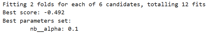

7. GloVe词向量 + XGboost

加载为 word->vector 的 embeddings_index = { }

文件中每行第一个词代表word 后面300维代表向量

# 1. 加载GloVe词向量
from tqdm import tqdm

embeddings_index = {}
with open('/kaggle/input/glove840b300dtxt/glove.840B.300d.txt', 'r', encoding='utf-8') as f:
    for line in tqdm(f):
        values = line.split()
        word = values[0]
        
        # 检查是否有足够的数值
        if len(values) == 301:  # 1个词 + 300个数字
            try:
                coefs = np.asarray(values[1:], dtype='float32')
                embeddings_index[word] = coefs
            except:
                continue

print('Found %s word vectors.' % len(embeddings_index))

将每个句子 tokenize分词；移除停用词 只保留字母；

所有词向量求和，并除以模长得到单位向量，作为句子的词向量

# 2. 转换文本为向量
from nltk.tokenize import word_tokenize
from nltk.corpus import stopwords
stop_words = stopwords.words('english')
def sent2vec(s):
    # 1. 文本预处理
    words = str(s).lower()           # 转换为小写
    words = word_tokenize(words)     # 分词：将句子拆分成单词列表
    words = [w for w in words if w not in stop_words]  # 移除停用词（如'the', 'is', 'and'等）
    words = [w for w in words if w.isalpha()]          # 只保留纯字母单词（移除数字和标点）
    
    # 2. 获取每个词的词向量
    M = []
    for w in words:
        try:
            M.append(embeddings_index[w])  # 从GloVe词典中获取词的300维向量
        except:
            continue  # 如果词不在GloVe词典中，跳过
    
    # 3. 处理空句子情况
    if len(M) == 0:
        return np.zeros(300)  # 如果没有有效词，返回300维零向量
    
    # 4. 组合词向量为句子向量
    M = np.array(M)           # 转换为numpy数组，形状为 (n_words, 300)
    v = M.sum(axis=0)         # 对所有词的向量求和，得到300维向量
    
    # 5. 向量归一化（单位化）
    norm = np.sqrt((v ** 2).sum())  # 计算向量的模长
    if norm > 0:
        v = v / norm  # 将向量除以其模长，得到单位向量
    else:
        v = np.zeros(300)  # 避免除以零
    
    return v

xtrain_glove = np.array([sent2vec(x) for x in tqdm(xtrain)])
xvalid_glove = np.array([sent2vec(x) for x in tqdm(xvalid)])

调用XGboost

import xgboost as xgb
clf = xgb.XGBClassifier(
    max_depth=7,            # 每棵树的最大深度，控制模型复杂度
    n_estimators=200,       # 树的数量（弱学习器的数量）
    colsample_bytree=0.8,   # 每棵树使用的特征比例，防止过拟合
    subsample=0.8,          # 每棵树使用的样本比例，防止过拟合
    n_jobs=10,              # 并行线程数，加速训练
    learning_rate=0.1,      # 学习率，控制每棵树的贡献程度
    random_state=42,        # 随机种子，确保结果可重现
    verbosity=1             # 输出训练信息（替代silent参数）
)
clf.fit(xtrain_glove, ytrain)
predictions = clf.predict_proba(xvalid_glove)

print ("logloss: %0.3f " % multiclass_logloss(yvalid, predictions))

8. GloVe词向量 + 深度学习

8.1 构建embedding_matrix 作为词嵌入层

由于神经网络拟合概率 将作家0 1 2转换为独热编码

# y转换为独热编码
from keras.utils import to_categorical
ytrain_enc = to_categorical(ytrain)
yvalid_enc = to_categorical(yvalid)

分词+相同长度填充；句子 -> 每个词对应token数值

from tensorflow.keras.preprocessing.text import Tokenizer
from tensorflow.keras.preprocessing.sequence import pad_sequences
token = Tokenizer(num_words=None)
max_len = 70

token.fit_on_texts(list(xtrain) + list(xvalid))
xtrain_seq = token.texts_to_sequences(xtrain)
xvalid_seq = token.texts_to_sequences(xvalid)

# zero pad the sequences
xtrain_pad = pad_sequences(xtrain_seq, maxlen=max_len)
xvalid_pad = pad_sequences(xvalid_seq, maxlen=max_len)

数值 -> 词向量 作为embedding

word_index = token.word_index
# create an embedding matrix for the words we have in the dataset
embedding_matrix = np.zeros((len(word_index) + 1, 300))
for word, i in tqdm(word_index.items()):
    embedding_vector = embeddings_index.get(word)
    if embedding_vector is not None:
        embedding_matrix[i] = embedding_vector

8.2 LSTM / 双头LSTM / GRU

循环层用 LSTM; Bi-directional LSTM ; GRU

冻结嵌入层 -> 空间Dropout -> 循环层 -> 全连接Dense层 -> 输出层三分类

from keras.models import Sequential
from keras.layers import Embedding, SpatialDropout1D, GRU, Dense, Dropout, Activation, LSTM, Bidirectional
from keras.callbacks import EarlyStopping

model = Sequential()

# 嵌入层：使用预训练的GloVe词向量
model.add(Embedding(
    len(word_index) + 1,      # 词汇表大小 + 1（为未知词预留）
    300,                      # 词向量维度（300维）
    weights=[embedding_matrix],  # 预训练的词向量矩阵
    input_length=max_len,     # 输入序列的最大长度
    trainable=False           # 冻结嵌入层，不更新词向量
))

model.add(SpatialDropout1D(0.3))

# model.add(LSTM(300, dropout=0.3, recurrent_dropout=0.3)) 若用LSTM
# model.add(Bidirectional(LSTM(300, dropout=0.3, recurrent_dropout=0.3))) 若用双头LSTM
# 下两行对应 GRU
model.add(GRU(300, dropout=0.3, recurrent_dropout=0.3, return_sequences=True))
model.add(GRU(300, dropout=0.3, recurrent_dropout=0.3))

model.add(Dense(1024, activation='relu'))
model.add(Dropout(0.8))

model.add(Dense(1024, activation='relu'))
model.add(Dropout(0.8))

# 输出层：3个神经元（对应3个类别），Softmax激活函数
model.add(Dense(3))  # 3分类问题
model.add(Activation('softmax'))

# 编译模型：使用分类交叉熵损失，Adam优化器
model.compile(loss='categorical_crossentropy', 
              optimizer='adam',
              metrics=['accuracy'])

# Fit the model with early stopping callback
earlystop = EarlyStopping(monitor='val_loss', min_delta=0, patience=3, verbose=0, mode='auto')
model.fit(xtrain_pad, y=ytrain_enc, batch_size=512, epochs=100, 
          verbose=1, validation_data=(xvalid_pad, yvalid_enc), callbacks=[earlystop])

8.3 预测+提交

texts_seq = token.texts_to_sequences(test.text.values)
texts_pad = pad_sequences(texts_seq, maxlen=max_len)
y_pred = model.predict(texts_pad)

sample[["EAP", "HPL", "MWS"]] = y_pred
sample.to_csv('submission.csv', index=False)