【机器学习与实战】分类与聚类算法：KNN鸢尾花分类

配套视频课程：www.bilibili.com/video/BV1iS...

一、关于数据集

Iris 数据集是机器学习中常用的数据集之一，也是 scikit-learn 中自带的数据集之一，由 Fisher 1936 收集整理，也称鸢尾花数据集。Iris 数据集是一个经典的多分类问题数据集，被广泛用于分类算法的性能评估、特征选择、特征提取和可视化等方面的研究。

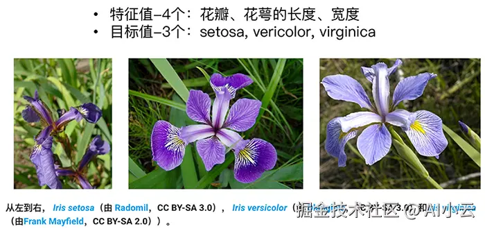
Iris 数据集包含了三种不同品种的鸢尾花 山鸢尾（Iris Setosa）、变色鸢尾（Iris Versicolour）和维吉尼亚鸢尾（Iris Virginica）
每个品种的各 50 个样本，总共 150 个样本
每个样本包含了**四个特征（花萼长度、花萼宽度、花瓣长度和花瓣宽度）**的测量值

利用Python代码加载数据集，并获取数据集相关信息：

python 复制代码

from sklearn.datasets import load_iris
# 获取鸢尾花数据集
iris = load_iris()
print("鸢尾花数据集的返回值：\n", iris)
# 返回值是一个继承自字典的Bench
print("鸢尾花的特征值:\n", iris["data"])
print("鸢尾花的目标值：\n", iris.target)
print("鸢尾花特征的名字：\n", iris.feature_names)
print("鸢尾花目标值的名字：\n", iris.target_names)
print("鸢尾花的描述：\n", iris.DESCR)

利用seaborn查看数据分布情况：

python 复制代码

import seaborn as sns
import matplotlib.pyplot as plt
import pandas as pd
from sklearn.datasets import load_iris
iris = load_iris()
# 把数据转换成dataframe的格式
iris_d = pd.DataFrame(iris['data'], columns = ['Sepal_Length', 'Sepal_Width', 'Petal_Length', 'Petal_Width'])
iris_d['Species'] = iris.target
col1 = 'Sepal_Width'
col2 = 'Sepal_Length'
sns.lmplot(x = col1, y = col2, data = iris_d, hue = "Species", fit_reg = False)
plt.xlabel(col1)
plt.ylabel(col2)
plt.show()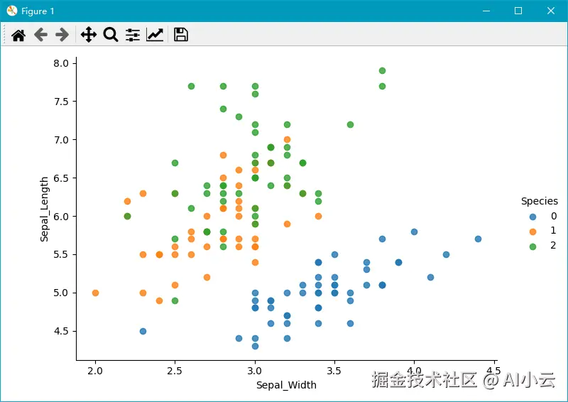

二、模型训练和评估

python 复制代码

from sklearn.datasets import load_iris
from sklearn.model_selection import train_test_split
from sklearn.preprocessing import StandardScaler
from sklearn.neighbors import KNeighborsClassifier
# 1.获取数据集
iris = load_iris()
# 2.数据基本处理
# x_train,x_test,y_train,y_test为训练集特征值、测试集特征值、训练集目标值、测试集目标值
x_train, x_test, y_train, y_test = train_test_split(iris.data, iris.target, test_size=0.2, random_state=22)
# 3.特征工程：标准化
transfer = StandardScaler()
x_train = transfer.fit_transform(x_train)
x_test = transfer.transform(x_test)    # 测试数据不能调用fit_transform否则将会不准确
# 4.机器学习(模型训练)
estimator = KNeighborsClassifier(n_neighbors=9)
estimator.fit(x_train, y_train)
# 5.模型评估
# 方法1：比对真实值和预测值
y_predict = estimator.predict(x_test)
print("预测结果为:\n", y_predict)
print("比对真实值和预测值：\n", y_predict == y_test)
# 方法2：直接计算准确率
score = estimator.score(x_test, y_test)
print("准确率为：\n", score)

输出结果为：

python 复制代码

预测结果为:
 [0 2 1 2 1 1 1 1 1 0 2 1 2 2 0 2 1 1 1 1 0 2 0 1 2 0 2 2 2 2]
比对真实值和预测值：
 [ True  True  True  True  True  True  True False  True  True  True  True
  True  True  True  True  True  True False  True  True  True  True  True
  True  True  True  True  True  True]
准确率为：
 0.9333333333333333

尝试一下，将n_neighbors参数从9修改为12，准确率上升到 0.9666666666666667，那么如何知道这是否是最优K值呢？

三、模型调优

1、K折交叉验证

交叉验证：将拿到的训练数据，分为训练和验证集。以下图为例：将数据分成4份，其中一份作为验证集。然后经过4次(组)的测试，每次都更换不同的验证集。即得到4组模型的结果，取平均值作为最终结果。又称4折交叉验证。

交叉验证可以让模型更加可信，但是不一定就能提升模型预测的准确率，所以使用网格搜索，可以继续提升其准确率。

python 复制代码

kf = KFold(n_splits=5)
for train, test in kf.split(x, y):
    x_train, x_test = x[train], x[test]
    y_train, y_test = y[train], y[test]
    estimator = KNeighborsClassifier(n_neighbors=7)
    estimator.fit(x_train, y_train)
    y_predict = estimator.predict(x_test)
    score = estimator.score(x_test, y_test)
    print("准确率为：\n", score)
# 也可以计算平均准确率，进而确定K折和n_neighbors的最佳效果

2、网格搜索

通常情况下，有很多参数是需要手动指定的（如k-近邻算法中的K值），这种叫超参数。但是手动过程繁杂，所以需要对模型预设几种超参数组合。每组超参数都采用交叉验证来进行评估。最后选出最优参数组合建立模型。

sklearn.model_selection.GridSearchCV(estimator, param_grid=None,cv=None)

解释：对估计器的指定参数值进行详尽搜索

参数：

estimator：估计器对象
param_grid：估计器参数(dict){"n_neighbors":[1,3,5]}
cv：指定几折交叉验证

方法：

fit：输入训练数据
score：准确率

结果分析：

bestscore__:在交叉验证中验证的最好结果
bestestimator：最好的参数模型
cvresults:每次交叉验证后的验证集准确率结果和训练集准确率结果

3、K值调优

使用GridSearchCV构建估计器

python 复制代码

from sklearn.datasets import load_iris
from sklearn.model_selection import train_test_split, GridSearchCV
from sklearn.preprocessing import StandardScaler
from sklearn.neighbors import KNeighborsClassifier
# 1、获取数据集
iris = load_iris()
# 2、数据基本处理 -- 划分数据集
x_train, x_test, y_train, y_test = train_test_split(iris.data, iris.target, test_size=0.2, random_state=5)
# 3、特征工程：标准化
# 实例化一个转换器类
transfer = StandardScaler()
# 调用fit_transform
x_train = transfer.fit_transform(x_train)
x_test = transfer.transform(x_test)
# 4、KNN预估器流程
# 4.1 实例化预估器类
estimator = KNeighborsClassifier()
# 4.2 模型选择与调优------网格搜索和交叉验证
# 准备要调的超参数
param_dict = {"n_neighbors": [1, 3, 5, 7, 9, 11]}
estimator = GridSearchCV(estimator, param_grid=param_dict, cv=5)
# 4.3 fit数据进行训练
estimator.fit(x_train, y_train)
# 5、评估模型效果
# 方法a：比对预测结果和真实值
y_predict = estimator.predict(x_test)
print("比对预测结果和真实值：\n", y_predict == y_test)
# 方法b：直接计算准确率
score = estimator.score(x_test, y_test)
print("直接计算准确率：\n", score)
print("在交叉验证中验证的最好结果：\n", estimator.best_score_)
print("最好的参数模型：\n", estimator.best_estimator_)
print("每次交叉验证后的准确率结果：\n", estimator.cv_results_)

输出结果为：

python 复制代码

比对预测结果和真实值：
 [ True  True  True  True  True  True  True  True  True  True  True False
  True  True  True  True  True  True  True  True  True  True  True False
  True  True  True  True  True  True]
直接计算准确率：
 0.9333333333333333
在交叉验证中验证的最好结果：
 0.975
最好的参数模型：
 KNeighborsClassifier(n_neighbors=9)    # 此处给出了最好的n_neighbors参数
每次交叉验证后的准确率结果：
 {'mean_fit_time': array([0.00060692, 0.00059123, 0.00059299, 0.00079851, 0.00040803,
       0.00060067]), 'std_fit_time': array([0.00049637, 0.00048293, 0.0004844 , 0.0003994 , 0.00049989,
       0.00049045]), 'mean_score_time': array([0.00278454, 0.00240145, 0.00259876, 0.00258627, 0.00259123,
       0.00219283]), 'std_score_time': array([0.00076474, 0.00049743, 0.00048247, 0.00049269, 0.00048831,
       0.00040145]), 'param_n_neighbors': masked_array(data=[1, 3, 5, 7, 9, 11],
             mask=[False, False, False, False, False, False],
       fill_value='?',
            dtype=object), 'params': [{'n_neighbors': 1}, {'n_neighbors': 3}, {'n_neighbors': 5}, {'n_neighbors': 7}, {'n_neighbors': 9}, {'n_neighbors': 11}], 'split0_test_score': array([1., 1., 1., 1., 1., 1.]), 'split1_test_score': array([1.        , 0.95833333, 0.95833333, 1.        , 1.        ,
       1.        ]), 'split2_test_score': array([0.95833333, 0.95833333, 0.95833333, 0.95833333, 0.95833333,
       0.95833333]), 'split3_test_score': array([0.95833333, 0.95833333, 0.95833333, 0.91666667, 0.95833333,
       0.95833333]), 'split4_test_score': array([0.91666667, 0.91666667, 0.91666667, 0.91666667, 0.95833333,
       0.95833333]), 'mean_test_score': array([0.96666667, 0.95833333, 0.95833333, 0.95833333, 0.975     ,
       0.975     ]), 'std_test_score': array([0.03118048, 0.02635231, 0.02635231, 0.0372678 , 0.02041241,
       0.02041241]), 'rank_test_score': array([3, 4, 4, 4, 1, 1])}

由上述输出结果可知，K设置为9时可以取得最好的效果。