一、全连接层神经元网络的缺点
|------|-------------------------------------------------------------------------------------------------------------------------------------------------------------------------------------|
| 点1 | 1.待优化的参数过多容易导致模型过拟合 全连接层的神经元网络参数个数(w和b): 例如:处理1000万像素的RGB彩色图,如果隐藏层为1000个神经元。那么参数仅w就是:1000x3x1000万=300亿个参数 |
| 缺点2 | 2.图片某个像素和周边的像素的组合才有意义。 全连接层去掉了''周边的概念',把所有像素平等的接入隐藏层(同样一幅图,像素互相调换位置后接入全连接层,调换前后对于全连接层是一样的,即使图片本身调换后完全变成一堆毫无意义的图片) |
| | |
| 改进意见 | 实际应用时会对原始图像进行特征提取,再把提取到的特征送给全连接层网络 |
二、卷积
卷积计算一般会用一个正方形的卷积核,按特定步长,在输入特征图上滑动。其覆盖的对应像素相乘相加再加上偏置项得到输出特征的一个像素点。
卷积计算可认为是一种有效提取图像特征的方法。
特点:
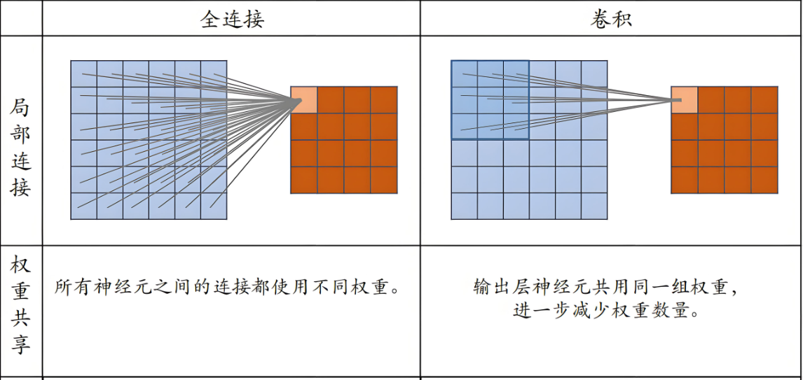
1.局部连接:每个神经元只与输入数据的一个局部区域连接,这符合图像数据的空间局部性
2.层次结构:能够自动学习从低级特征(边缘、角点)到高级特征(物体部分、整体)的表示
3.平移不变性:通过池化操作,网络对输入图像的小范围平移具有不变性
4.参数共享:卷积层使用相同的卷积核在输入数据上滑动,大大减少了参数数量
【例1】3*3*1卷积核有:3x3+1=10个参数
3x3x3立体卷积核有:3x3x3+1=28个参数
5x5x3卷积核每个核有:76个参数
2.1 卷积
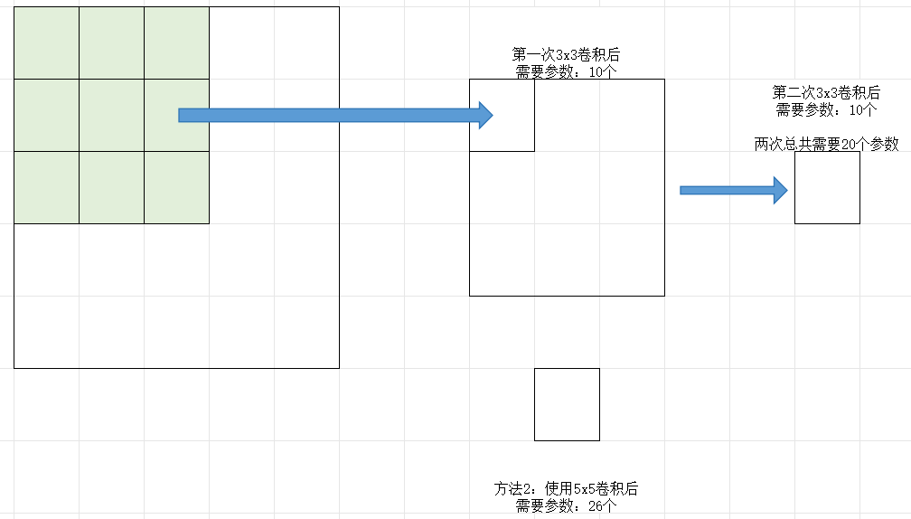
两层3x3的卷积核(参数20个)和一层5x5(参数26个)的卷积核特征提取能力是一样的。一般来讲2层3x3的卷积核优于一层5x5的。
tf.keras.layers.Conv2D(filters=6, //卷积核个数
kernel_size=(5,5),        //卷积核尺寸
strides=1,                //滑动步长
padding='same',
activation='relu' or 'sigmoid' or 'softmax' //如果之后还有批标准化操作,则此处不填写。
)           //全零填充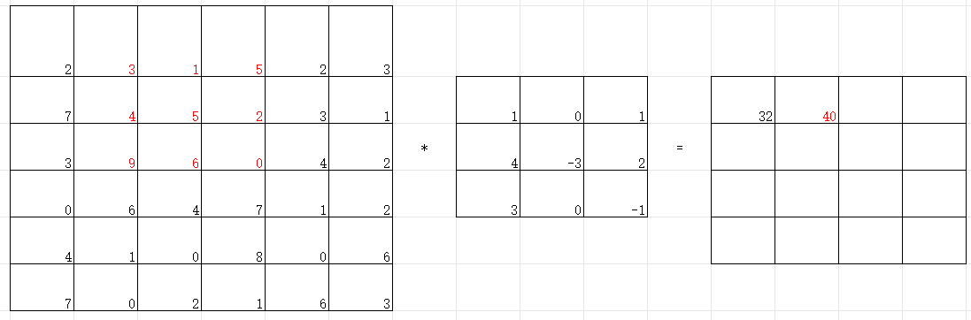
2.2 填充
padding='SAME'(全0填充),那么输出的尺寸 = 输入尺寸 / 步长
或者padding='VALID'(不全0填充),那么输出的尺寸 = (入厂 - 核长+1)/步长。
2.3 批标准化
标准化:使数据符合0均值,1为标准差的分布
批标准化:对一小批数据(batch),做标准化处理
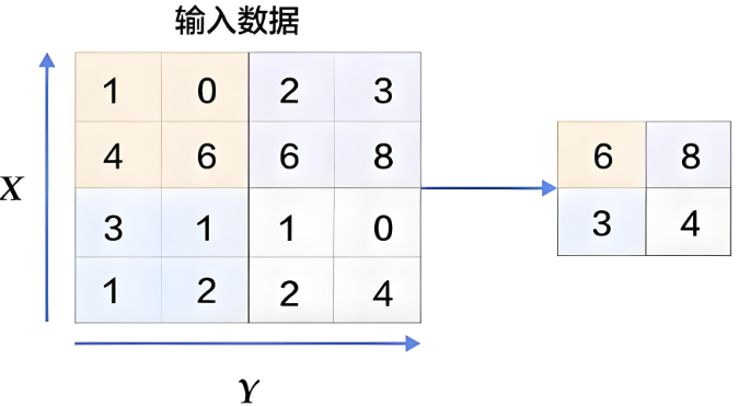
2.4 池化
用于减少特征数据量,最大值池化可提取图片纹理,均值池化可保留背景特征。
最大化池化示意图
tf.keras.layers.MaxPool2D(        //最大化池化
pool_size=(2,2),  //池化核尺寸
strides=2,        //池化步长
padding='same')   //默认valid, 全零填充'same'

tf.keras.layers.AveragePooling2D //均值池化
2.5 dropout舍弃
将一部分神经元网络按照一定概率从神经网络中暂时舍弃,使用时,被舍弃的神经元恢复连接。
tf.keras.layers.Dropout(0.2) //舍弃的比例
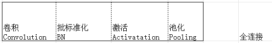
三、卷积神经网络
借助卷积核提取特征后,送入全连接网络。
【例1】先加载cifar10数据集
一般通过下面两行代码即可。
cifar10 = tf.keras.datasets.cifar10
(x_train, y_train), (x_test, y_test) = cifar10.load_data()
也可以通过通过下载数据包,自己编写代码进行加载
python
import pickle

from keras.src.layers import Conv2D
from matplotlib import pyplot as plt
from keras.src.layers import  Activation,  Dropout, Flatten, Dense
from tensorflow.python.keras.models import Model
from keras.src.layers import BatchNormalization
from tf_keras.src.layers import MaxPool2D
import numpy as np

def load_cifar10():

    # 加载训练数据
    train_images = []
    train_labels = []

    for i in range(1, 6):
        batch_file = f'./cifar-10-batches-py/data_batch_{i}'
        with open(batch_file, 'rb') as f:
            batch_data = pickle.load(f, encoding='bytes')
            # 注意:CIFAR-10使用bytes键
            train_images.append(batch_data[b'data'])
            train_labels.append(batch_data[b'labels'])

    # 合并训练数据
    train_images = np.vstack(train_images)
    train_labels = np.hstack(train_labels)

    # 加载测试数据
    test_file = './cifar-10-batches-py/test_batch'
    with open(test_file, 'rb') as f:
        test_data = pickle.load(f, encoding='bytes')
        test_images = test_data[b'data']
        test_labels = np.array(test_data[b'labels'])

    return (train_images, train_labels), (test_images, test_labels)


def preprocess_cifar10_data(train_images, train_labels, test_images, test_labels):
    """
    预处理CIFAR-10数据
    """
    # 重塑图像数据 (50000, 3072) -> (50000, 32, 32, 3)
    # CIFAR-10数据的原始格式是每行3072个值,前1024个是红色通道,接着是绿色,最后是蓝色
    train_images = train_images.reshape((-1, 3, 32, 32)).transpose(0, 2, 3, 1)
    test_images = test_images.reshape((-1, 3, 32, 32)).transpose(0, 2, 3, 1)

    # 归一化到0-1范围
    train_images = train_images.astype('float32') / 255.0
    test_images = test_images.astype('float32') / 255.0


    return train_images, train_labels, test_images, test_labels

# 使用示例
(train_images, train_labels), (test_images, test_labels) = load_cifar10()

# 类别名称
class_names = ['airplane', 'automobile', 'bird', 'cat', 'deer',
               'dog', 'frog', 'horse', 'ship', 'truck']

# 预处理数据
x_train, y_train, x_test, y_test = preprocess_cifar10_data(
    train_images, train_labels, test_images, test_labels
)


fig = plt.figure(figsize=(20, 2))
plt.set_cmap('gray')
# 显示原始图片
for i in range(0, len(x_train[:12])):
    ax = fig.add_subplot(1, 12, i + 1)
    ax.imshow(x_train[i])
    ax.set_title(y_train[i])
fig.suptitle('Subset of Original Training Images', fontsize=20)
plt.show()


print('x_train[0]:\n',x_train[0])
print('y_train[0]:\n',y_train[0])
print('x_test.shape',x_test.shape)

exit()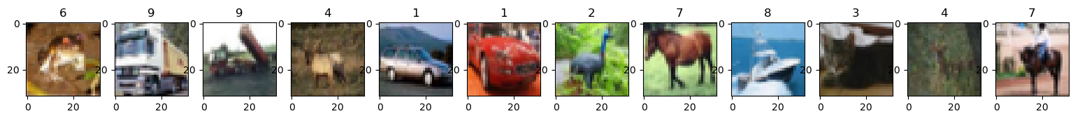
【例2】用卷积网络进行训练和保存
注意下面代码可以把训练后的模型保存参数,但是确不能正确的读取该参数。参数保存还需要完善。
python
import pickle

import keras
import tensorflow as tf
import os
import numpy as np
from keras import Model
from keras.src.layers import Conv2D, BatchNormalization, Activation, Dropout, Flatten, Dense
from matplotlib import pyplot as plt
from tf_keras.src.layers import MaxPool2D


def load_cifar10():
    # 加载训练数据
    train_images = []
    train_labels = []

    for i in range(1, 6):
        batch_file = f'./cifar-10-batches-py/data_batch_{i}'
        with open(batch_file, 'rb') as f:
            batch_data = pickle.load(f, encoding='bytes')
            # 注意:CIFAR-10使用bytes键
            train_images.append(batch_data[b'data'])
            train_labels.append(batch_data[b'labels'])

    # 合并训练数据
    train_images = np.vstack(train_images)
    train_labels = np.hstack(train_labels)

    # 加载测试数据
    test_file = './cifar-10-batches-py/test_batch'
    with open(test_file, 'rb') as f:
        test_data = pickle.load(f, encoding='bytes')
        test_images = test_data[b'data']
        test_labels = np.array(test_data[b'labels'])

    return (train_images, train_labels), (test_images, test_labels)


def preprocess_cifar10_data(train_images, train_labels, test_images, test_labels):
    """
    预处理CIFAR-10数据
    """
    # 重塑图像数据 (50000, 3072) -> (50000, 32, 32, 3)
    # CIFAR-10数据的原始格式是每行3072个值,前1024个是红色通道,接着是绿色,最后是蓝色
    train_images = train_images.reshape((-1, 3, 32, 32)).transpose(0, 2, 3, 1)
    test_images = test_images.reshape((-1, 3, 32, 32)).transpose(0, 2, 3, 1)

    # 归一化到0-1范围
    train_images = train_images.astype('float32') / 255.0
    test_images = test_images.astype('float32') / 255.0

    return train_images, train_labels, test_images, test_labels

# 使用示例
(train_images, train_labels), (test_images, test_labels) = load_cifar10()

# 类别名称
class_names = ['airplane', 'automobile', 'bird', 'cat', 'deer',
               'dog', 'frog', 'horse', 'ship', 'truck']

# 预处理数据
x_train, y_train, x_test, y_test = preprocess_cifar10_data(
    train_images, train_labels, test_images, test_labels
)


np.set_printoptions(threshold=np.inf)


class Baseline(Model):
    def __init__(self):
        super().__init__()
        self.trainable = True  # 实例属性赋值
        self.c1 = Conv2D(filters=6, kernel_size=(5, 5), padding='same')  # 卷积层
        self.b1 = BatchNormalization()  # BN层
        self.a1 = Activation('relu')  # 激活层
        self.p1 = MaxPool2D(pool_size=(2, 2), strides=2, padding='same')  # 池化层
        self.d1 = Dropout(0.2)  # dropout层

        self.flatten = Flatten()
        self.f1 = Dense(128, activation='relu')
        self.d2 = Dropout(0.2)
        self.f2 = Dense(10, activation='softmax')

    def call(self, x):
        x = self.c1(x)
        x = self.b1(x)
        x = self.a1(x)
        x = self.p1(x)
        x = self.d1(x)

        x = self.flatten(x)
        x = self.f1(x)
        x = self.d2(x)
        y = self.f2(x)
        return y

model = Baseline()


checkpoint_save_path = "./checkpoint/Baseline.keras"
if os.path.exists(checkpoint_save_path):
    print('-------------load the model-----------------')
    #model = keras.models.load_model(checkpoint_save_path,custom_objects={
    #    'Baseline': Baseline  # 键为保存模型时记录的自定义模型类名
    #})

model.compile(optimizer='adam',
              loss=keras.losses.SparseCategoricalCrossentropy(from_logits=False),
              metrics=['sparse_categorical_accuracy'])

history = model.fit(x_train, y_train, batch_size=32, epochs=3, validation_data=(x_test, y_test), validation_freq=2)

model.summary()
model.save(checkpoint_save_path)
pred_x = x_train[0][tf.newaxis,...]
value= np.max(np.argmax( model.predict(pred_x),axis=1))
print(value)

# print(model.trainable_variables)
file = open('./weights.txt', 'w')
for v in model.trainable_variables:
    file.write(str(v.name) + '\n')
    file.write(str(v.shape) + '\n')
    file.write(str(v.numpy()) + '\n')
file.close()

###############################################    show   ###############################################

# 显示训练集和验证集的acc和loss曲线
acc = history.history['sparse_categorical_accuracy']
val_acc = history.history['val_sparse_categorical_accuracy']
loss = history.history['loss']
val_loss = history.history['val_loss']

plt.subplot(1, 2, 1)
plt.plot(acc, label='Training Accuracy')
plt.plot(val_acc, label='Validation Accuracy')
plt.title('Training and Validation Accuracy')
plt.legend()

plt.subplot(1, 2, 2)
plt.plot(loss, label='Training Loss')
plt.plot(val_loss, label='Validation Loss')
plt.title('Training and Validation Loss')
plt.legend()
plt.show()