目录
[1.1 引入](#1.1 引入)
[1.2 决策树的构建](#1.2 决策树的构建)
[1.3 常见算法介绍](#1.3 常见算法介绍)
[1.3.1 ID3(信息增益)](#1.3.1 ID3(信息增益))
[1.3.2 C4.5(信息增益率)](#1.3.2 C4.5(信息增益率))
[1.3.3 CART(基尼系数)](#1.3.3 CART(基尼系数))
[1.3.4 算法对比](#1.3.4 算法对比)
[1.4 评估方法](#1.4 评估方法)
[2.1 案例分析](#2.1 案例分析)
[2.2 实现流程](#2.2 实现流程)
[3.1 C++实现](#3.1 C++实现)
[3.1.1 实现环境](#3.1.1 实现环境)
[3.1.2 完整代码](#3.1.2 完整代码)
[3.1.3 核心代码讲解](#3.1.3 核心代码讲解)
[3.1.4 结果展示](#3.1.4 结果展示)
[3.2 Python实现](#3.2 Python实现)
[3.2.1 实现环境](#3.2.1 实现环境)
[3.2.2 完整代码](#3.2.2 完整代码)
[3.2.3 核心代码讲解](#3.2.3 核心代码讲解)
[3.2.4 结果展示](#3.2.4 结果展示)
一、决策树原理
1.1 引入
在生活中,我们不少遇到类似这样的测试------让你回答几个问题,从而得到答案,典型的代表有海龟汤、MBTI测试、生物分类等等。这是人类预测某个东西的常用方法,像这样的测试,在机器学习中被抽象出来利用,形成了决策树这种算法。
1.2 决策树的构建
由引入可知,我们构建的决策树必须能够满足根据先提出的问题给出的答案推测结果,甚至需要进一步提问并循环,直到能推测结果。然而,我们很难通过编程的方式,把整个算法动态的描述出来。
所以,决策树算法需要已知每个问题对应的答案后面的问题是什么,且根据下一个问题再次"提问",再次得到答案,循环这个过程,直到得到的答案后面的是结果。
这样的算法思路,很适合使用树的结构来管理,因此,决策树是一个以树为数据结构的模型。现在的问题变成了,我们要如何选择合适的"问题"作为第一个提问的"问题",以及通过这个问题得到的答案后面是跟着新的问题还是预测的结果。
为了解决这个问题,我们先回到决策树构建的构建逻辑上:人类的分类思维是把具有相同的一个或多个特征的物品归为一类,并且哪个物品越符合这些特征,就越可能是这个类,所以我们需要提前知道样本的标签,因此这个算法是有监督学习。
通过构建的决策树的准确率反向验证算法效果是可行的方案,前人就是借助"熵"的概念,设计出了出多个高效的算法,接下来我们逐一介绍。
1.3 常见算法介绍
首先说明为什么需要使用这些算法提取特征:为了得到准确率最高的决策树模型,我们需要提高决策树的纯度(如下),每次选择让数据集的纯度提升最大的特征,这样整个决策树的纯度提升效率最高,分类效果最好,同时模型复杂度更低、训练速度更快。
熵 ,在决策树中用于描述数据集的不确定性 (混乱程度),是用来决定特征优先级 和决策树分列时机的重要指标。
纯度 ,用于描述数据集中样本归属于同一类别的集中程度 ,换句话说,就是同一个类别的占比越高,数据集的纯度越高。纯度与熵的概念是互补的,是衡量数据集数据类别集中程度的核心指标。
1.3.1 ID3(信息增益)
信息增益是基于熵的指标的算法,用来衡量"一个特征作为分类标准,数据集的不确定性减少的程度" 。其中,条件熵 (根据特征分类得到的熵)越小,信息增益越大,对应数据集的纯度提升越明显。
熵的计算公式,D是某一特征一个类别划分出来的数据集,y是这个数据集对应的标签数量,p_k是某种标签的占比:
信息增益的计算公式,计算总的熵,减去某一特征分出来数据集的条件熵,v是特征a的某个类别,|D|是数据集的样本数量:
计算每个特征的信息增益,选择其中信息增益最大的那一个作为当前的根节点分类。
1.3.2 C4.5(信息增益率)
信息增益率,是在原来信息增益的基础上进行优化。
信息增益的缺陷
为什么我们要优化ID3呢?研究表明,信息增益更倾向于选择类别多的特征 。例如一共数据集一共有10个样本,里面有颜色这种特征,颜色特征的类别分别是不同的颜色名称,每个类别下只有一个样本,纯度达到100%,根据算法,肯定选择这个特征作为父节点。然而,在这里,颜色特征没有什么实际意义,选择的特征反而会提高树高 。根据奥卡姆剃刀,我们希望这样的情况越少出现越好。
信息增益率的原理
信息增益率,是信息增益与分裂信息的比值 。这样的处理叫作规范化、正则化,分裂信息是特征自身的熵,当特征的类别越多时,特征的不确定性越高,自然熵越高,对信息增益进行一定程度的惩罚 ,让算法更不容易选择没有意义的特征。
分裂信息计算公式,和熵的计算公式一样:
信息增益率计算公式:
但是,这样的算法反而对类别较少的特征有所偏好。
1.3.3 CART(基尼系数)
基尼系数,又称基尼不纯度,描述"从数据集中随机抽取两个样本,它们属于不同类别的概率 "。概率越低,数据集类别越集中,纯度越高。
总体基尼系数公式,P是某一特征一个类别划分出来的数据集,K是数据集的标签数,p_k是某个标签的占比:
条件基尼系数公式,
相较于前面的信息增益和增益率,计算复杂度要更低,没有对数运算
1.3.4 算法对比
|--------|-----------------------|-----------------|-------------------|
| 对比维度 | ID3 | C4.5 | CART |
| 支持特征类型 | 离散 | 离散+连续 | 离散+连续 |
| 节点分裂 | 多叉 | 多叉 | 二叉 |
| 内置剪枝处理 | 不支持 | 后剪枝 | 前剪枝+后剪枝 |
| 优点 | 算法简单易懂 | 支持连续特征,泛化能力强 | 计算高效,二叉树结构简洁,工程友好 |
| 缺点 | 偏向多类别特征,容易过拟合,计算复杂度较高 | 偏向少类别特征,计算复杂度较高 | 多分类问题需要间接实现 |
| 使用场景 | 小规模、处理离散特征 | 中大型规模,需要较高的泛化能力 | 大规模,用于工程落地 |
1.4 评估方法
本文使用准确率、精确率、召回率和混淆矩阵评估模型的好坏。
二、实战案例
原型
简化
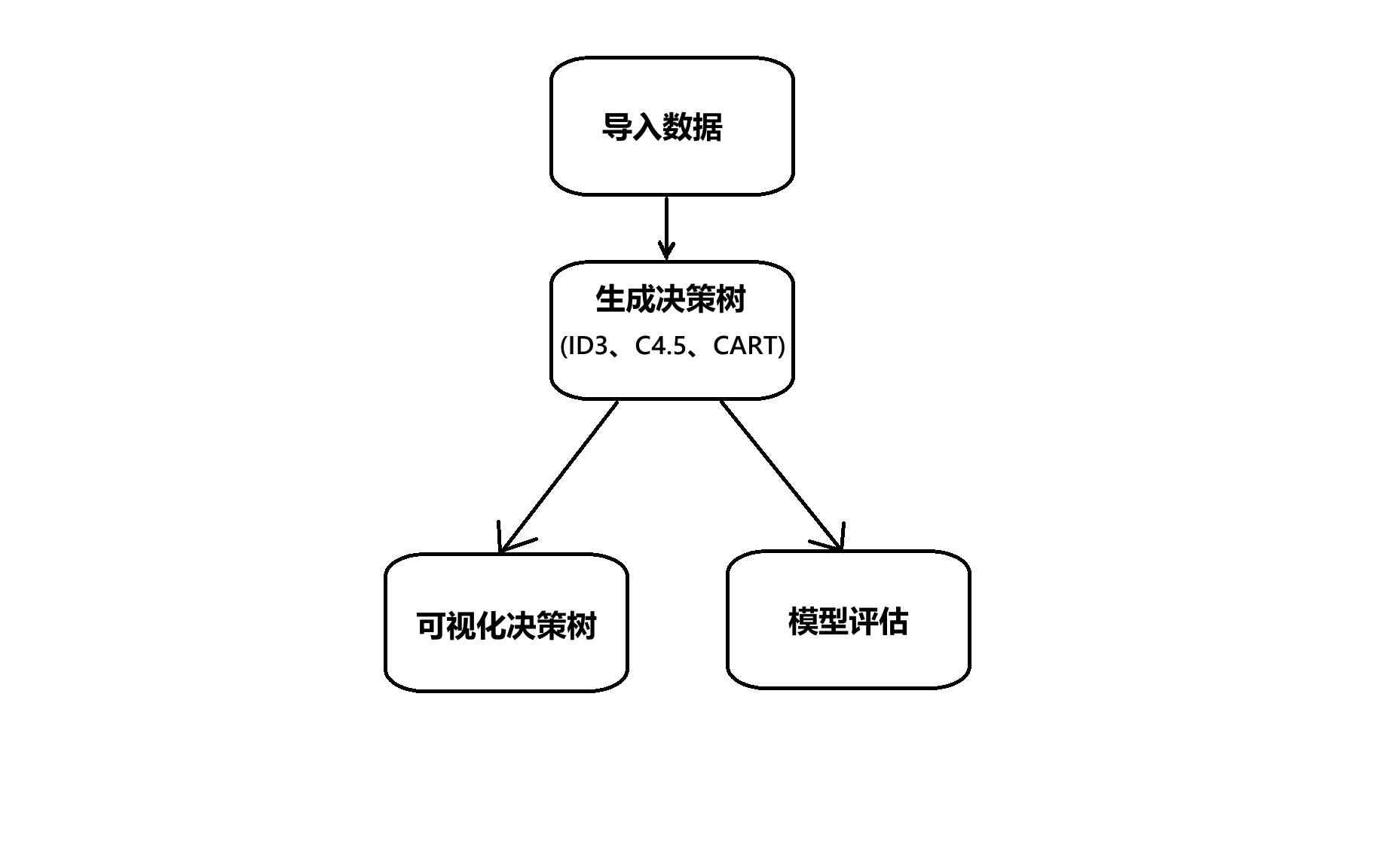
根据数据集,生成决策树
2.1 案例分析
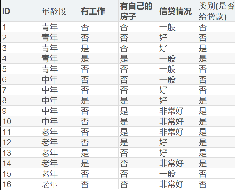
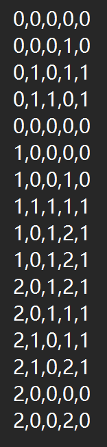
数据集的前四项是特征,最后一项是标签。我们需要先将数据导入,使用算法生成决策树,再用各种评估指标评估。就是这么简单。本文将三种算法都实现了,并可视化了决策树。(由于数据集太小了,这里就不使用K折交叉验证泛化能力了)
2.2 实现流程
三、代码实现
3.1 C++实现
3.1.1 实现环境
集成开发环境------VS2022
可视化库------matplot++
可视化环境------gnuplot
3.1.2 完整代码
代码行数超500行,到github仓库上下载吧!
小编使用premake来管理项目。拿到项目后,到解决方案文件夹中,双击"generatePrj.bat"批处理文件,即可配置好项目,注意**:Windows系统上才能使用我项目中的批处理文件**;gnuplot环境还需要自行配置

3.1.3 核心代码讲解
模型评估和上一次类似,这里就不重复讲解了
结构体
数据的结构体,features动态存入多个特征,tag存入标签
cpp
struct Data
{
	std::vector<int> features;
	int tag;
};
树节点的结构体,val存放这个节点父节点特征中选择的值;feature存放它自己的值;is_leaf存放这个节点的状态------是否为叶子节点;DecisionTreeNode构造函数(C++中struct也可以在内部实现函数)用于初始化节点;~DecisionTreeNode析构函数用于释放堆区内存;operator<< 符号重载,用于打印数据,下面的to_string函数类似,对应python的魔术方法__str__。
cpp
struct DecisionTreeNode
{
	int val; // value From parent-node's feature
	int feature; // feature type
	bool is_leaf;
	std::vector<DecisionTreeNode*> Children;

	DecisionTreeNode(int value, int f, bool leaf = false,
		std::vector<DecisionTreeNode*> children = std::vector<DecisionTreeNode*>())
		: val(value), feature(f), is_leaf(leaf), Children(children)
	{
	}

	~DecisionTreeNode()
	{
		for (auto& child : Children)
			delete child;

		Children.clear();
	}

	friend std::ostream& operator<< (std::ostream& os, const DecisionTreeNode& node)
	{
		if (node.is_leaf)
			os << "result: " << node.val;
		else
			os << "feature: " << node.feature;
		return os;
	}

	std::string to_string() const
	{
		std::ostringstream oss;
		oss << *this;
		return oss.str();
	}
};
导入数据
cpp
std::vector<int> split(std::string& s, char div)
{
	std::vector<int> tokens;
	std::string token;
	std::istringstream tokenStream(s);

	while (std::getline(tokenStream, token, div))
		tokens.push_back(std::stoi(token));

	return tokens;
}导入数据的部分就不提了,直接for循环getline,想简单一点 就有几个特征写几个成员 ,想要动态 的可以先分割一行的字符串提取出一个列表,使用上面的分割函数实现这个效果。
类numpy函数
cpp
template<bool return_counts = false>
auto unique(const std::vector<int>& buffer, bool sort = true)
{
	std::unordered_map<int, int> map;
	for (int type : buffer)
		map[type]++;

	std::vector<int> genres;
	genres.reserve(map.size());
	for (const auto& m : map)
		genres.push_back(m.first);
	if (sort)
		std::sort(genres.begin(), genres.end());

	if constexpr (return_counts)
	{
		std::vector<int> counts;
		counts.reserve(genres.size());
		for (int val : genres)
			counts.push_back(map[val]);
		return std::make_pair(genres, counts);
	}
	else
		return genres;
}matplot++将C++提升到C++17,这意味着不用考虑C++11等其他更早的C++版本标准,所以我们使用if-constexpr语句反而更加通用了。如标题所述,这个函数是个高仿numpy.unique的函数,我们要实现的功能是统计vector<int>中出现的不同类别的列表以及对应的个数 ,先使用unordered_map哈希表来存放数据,再对key值排序,最后获取对应value值完成统计,可选是否需要value值列表。
cpp
std::vector<int> bincount(const std::vector<int>& buffer)
{
	return unique<true>(buffer).second;
}
外放接口,模拟numpy.bincount函数,只返回value值列表。
cpp
std::vector<bool> in(const std::vector<int>& buffer, int element)
{
	std::vector<bool> inlist;
	inlist.reserve(buffer.size());
	for (auto& val : buffer)
		inlist.push_back(val == element);

	return inlist;
}
获取布尔列表,为提取某个特征中同一类型样本的列表做准备
cpp
std::vector<int> splitlist(const std::vector<bool>& idxlist, const std::vector<int>& source)
{
	std::vector<int> dist;
	for (int i = 0; i < idxlist.size(); ++i)
	{
		if (idxlist[i])
			dist.push_back(source[i]);
	}

	return dist;
}

std::vector<std::vector<int>> splitlist(const std::vector<bool>& idxlist, std::vector<std::vector<int>> source)
{
	int offset = 0;
	for (int i = 0; i < idxlist.size(); ++i)
	{
		if (!idxlist[i])
		{
			for (auto& s : source)
			{
				s.erase(s.begin() + i - offset);
			}
			offset++;
		}
	}

	return source;
}生成新列表,根据数据类型不同分为了两个函数,一个是以行 为特征(前者),一个是以列 为特征(后者)。需要去掉的是样本(前者去掉列 ,后者去掉行)。
指标计算函数
cpp
double Ent(const std::vector<int>& fqcy, int num)
{
	if (num <= 0)
		CatchErr("Ent: 除零错误");
	double sum = 0.0;
	for (auto& f : fqcy)
	{
		if (f == 0) continue;
		double prob = double(f) / num;
		sum += prob*log(prob)/log(2);
	}
	return -sum;
}遍历值列表,计算每一个类别的占比 ,套用公式计算,使用累加器sum累加每个占比的计算结果 ,最后返回信息熵计算的结果 。由于信息增益率 和信息增益都是使用这个核心的计算公式,下文使用信息增益率生成树时,直接复用这个函数,不另外写一个函数。
cpp
double Gini(const std::vector<int>& fqcy, int num)
{
	if (num <= 0)
		CatchErr("Gini: 除零错误");
	double sum = 1.0;
	for (auto& f : fqcy)
	{
		if (f == 0) continue;
		double prob = double(f) / num;
		sum -= prob*prob;
	}
	return sum;
}和信息熵一样的遍历 和得到占比 的方式,直接使用prob*prob,算平方,同样使用sum累加每个占比的计算结果。
分裂函数
cpp
std::vector<double> branch(std::vector<std::vector<int>>& features, std::vector<int>& tags,
double(classifier)(const std::vector<int>&, int), bool ratio = false)
{
	if (features.empty())
		CatchErr("branch: 数据为空");
	int sample = tags.size();
	if (sample <= 0)
		CatchErr("branch: 数据无效");

	double base_value = (classifier == Ent ? classifier(bincount(tags), sample) : -1);
	std::vector<double> values;
	values.reserve(tags.size());
	for (auto& feature : features)
	{
		auto& [tag, cnt] = unique<true>(feature);
		int sz = tag.size();
		double rate = ratio ? classifier(cnt, sample) : 1;
		double count_value = 0.0;
		for (int i = 0; i < sz; ++i)
		{
			int t = tag[i];
			int c = cnt[i];
			auto sublist = splitlist(in(feature, t), tags);
			count_value += ((double)c / sample) * classifier(bincount(sublist), c);
		}
		values.push_back(base_value >= 0 ? (base_value - count_value)/rate : count_value);
	}

	return values;
}三种算法格外实现过程格外的相似,这里使用一个函数将三个算法的核心思路凝练出来。思路:判断分类器类型,计算总的指标 ,遍历每一列特征(已经使用转置函数transform处理了),获取特征的类型和数量 ,将同一类别的样本整理出新的列表 ,计算指标,将所有这个特征的指标加权 (按类型占比)地累加起来 ,留到最后处理。
Gain 需要的是使用总指标减去累加器;GainRatio 需要的是除了获取Gain外,需要使用rate对信息增益进行惩罚,我们可以使用ratio这个标记区分,标记为假,rate为1,除了相当于没除,为真就是正常惩罚 ;Gini 不需要再操作了。这样就能获取到所有特征的某一种指标了。
外放接口
cpp
std::vector<double> Gain(std::vector<std::vector<int>>& features, std::vector<int>& tags)
{
	return branch(features, tags, Ent);
}
std::vector<double> GainRatio(std::vector<std::vector<int>>& features, std::vector<int>& tags)
{
	return branch(features, tags, Ent, true);
}
std::vector<double> CART(std::vector<std::vector<int>>& features, std::vector<int>& tags)
{
	return branch(features, tags, Gini);
}
生成决策树函数
通过前面大量函数的准备,终于到了生成决策树的时候。
cpp
DecisionTreeNode* CreateDecistionTree(std::vector<std::vector<int>> features, std::vector<int> tags,
	std::vector<int> idxlist, ClassifierFunc classifier)
{
	if (unique(tags).size() == 1)
		return new DecisionTreeNode(tags[0], -1, true);
	if (idxlist.size() == 0)
	{
		auto taglist = bincount(tags);
		int max_tag = std::max_element(taglist.begin(), taglist.end()) - taglist.begin();
		return new DecisionTreeNode(max_tag, -1, true);
	}

	auto val = classifier(features, tags);
	int idx = (classifier == Gain || classifier == GainRatio ? std::max_element(val.begin(), val.end()) : std::min_element(val.begin(), val.end())) - val.begin();
	if (idx >= features.size())
		CatchErr("CreateDecisionTree: 最大值索引超过数据集大小");

	std::vector<int> values(features[idx]);
	auto typenumlist = unique(values);

	features.erase(features.begin() + idx);
	std::vector<int> newlist(idxlist);
	newlist.erase(newlist.begin() + idx);

	std::vector<DecisionTreeNode*> children;
	children.reserve(values.size());
	for (int t : typenumlist)
	{
		std::vector<bool> sublist = in(values, t);
		auto sub_features = splitlist(sublist, features);
		auto sub_tags = splitlist(sublist, tags);
		auto child = CreateDecistionTree(sub_features, sub_tags, newlist, classifier);
		child->val = t;
		children.push_back(child);
	}

	return new DecisionTreeNode(idx, idxlist[idx], false, children);
}先获取指标列表,从中获取选择最佳指标 (最大值或最小值的下标),获取最佳指标对应的特征所在的列表 (这里是所在的行),从数据集和特征列表(idxlist)去掉最佳指标对应的特征相关的信息 ,遍历当前最佳特征的所有类别,取出所有属于这一类的样本及其对应的标签,,进入递归。
在递归中,重复上述内容构建作为根节点的子节点,直到没有特征可用 或者是标签列表 (tags)只有唯一的预测结果 ,前者需要选择最多数量的标签作为预测结果放在val中,后者直接把tags中的一个元素取出来存就行了;将feature设置为-1 ,存放不存在的类 ,防止初始化信息缺少;显式设置is_leaf,提高可读性。
结束递归后,记录子节点的类别(child->val),生成一个子节点的列表,形成n叉树。整棵决策树的根节点的val值是无效的,同样是为了初始化补上的数据。
可视化函数
上一篇文章有提及可视化热力图,这里就不重复了,主要讲一下如何使用matplot++可视化的思路。由于函数写得太大了,所以这里就不展示了,在src/plotshow.cpp中。
matplot++本身没有可以传入一个树可视化出一个树图的函数,不支持。我们需要计算图形位置,并使用matplot++内置的线(使用plot提供一段定义域较小的直线方程)、矩形等,本项目使用矩形表示非叶子节点,用圆形表示叶子节点,matplot++同样没有圆形,所以在项目中只能看到小编自己写的调用plot函数生成的圆。
位置需要获取整个树的高度,这里使用层序遍历获取。得到树的高 后,我们可以算出每一层的位置y 应该是多少(预计的大小除以树高),x则是从定义0.5为根节点的水平位置开始 ,之后每一层围绕父节点的水平位置,设置一个越往深处越小的数值 (项目中是branchGap),计算这个父节点n个孩子占的水平位置的距离**(n-1)*branchGap** ,父节点减去距离的一半是子节点的起始位置 ,然后接下来的每一个子节点比它左边的兄弟多branchGap的水平距离。循环这个计算根据父节点计算子节点的操作,我们就能得到key表示节点名称、value表示节点位置(x、y)的unordered_map字典 ,以上操作除了计算位置,我们也可以同步画线,配上特征类别字幕。
最后遍历整个字典,将矩形和圆形画上,配上特征类别的字幕字幕。一个决策树的可视化就完成了。
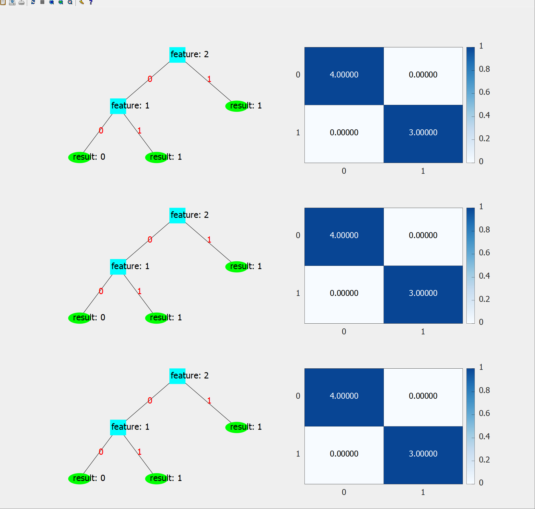
3.1.4 结果展示
3.2 Python实现
3.2.1 实现环境
python:集成开发环境------Pycharm,数学库------numpy,可视化库------matplotlib
3.2.2 完整代码
python
import copy
import numpy as np
import matplotlib.pyplot as plt
from matplotlib.patches import Rectangle, Circle, ConnectionPatch
from numpy.f2py.auxfuncs import throw_error
from numpy.ma.core import zeros
plt.rcParams['font.sans-serif']=['SimHei'] # 用来正常显示中文标签
plt.rcParams['axes.unicode_minus'] = False # 用来显示负号
class DecisionTreeNode:
def __init__(self, val, feature, is_leaf=False, children=None):
self.val = val
self.feature = feature
self.is_leaf = is_leaf
self.children = children if children is not None else []
def __str__(self):
if self.is_leaf:
return f"Result: {self.val}"
return f"Node: {self.feature}"
def load_data(filepath):
data = []
tag = []
with open(filepath, 'r', encoding="utf-8") as f:
for line in f:
line = line.strip()
if not line:
continue
parts = line.split(',')
if len(parts) != 5:
print(f"特征数据无法转换:{line}")
continue
data.append([int(x) for x in parts[:-1]])
tag.append(int(parts[-1]))
data_np = np.array(data, dtype=np.int32)
tag_np = np.array(tag, dtype=np.int32)
return data_np, tag_np
def count_ent(cnt, num):
prob = np.array(cnt, dtype=float)
prob /= num
prob = prob[prob>0]
return -np.sum(prob*np.log2(prob))
def get_gain(datas: np.ndarray, tags: np.ndarray, ratio = False):
sample_num, feature_num = datas.shape
base_ent = count_ent(np.bincount(tags), sample_num)
print(feature_num)
# print(f"base_ent: {base_ent}")
gains = []
feature_ent = []
for r in datas.T:
tag, cnt = np.unique(r, return_counts=True)
count_accuracy = 0.0
for t, c in zip(tag, cnt):
mask = tags[r == t]
count_accuracy += (c/sample_num) * count_ent(np.bincount(mask), c)
print(f"条件熵:{count_accuracy},信息增益:{base_ent-count_accuracy}")
if ratio:
feature_ent.append(count_ent(cnt, sample_num))
gains.append(base_ent - count_accuracy)
gains = np.array(gains)
if ratio:
gain_ratios = gains/np.array(feature_ent)
return gain_ratios
else:
return gains
def count_gini(cnt, num):
prob = np.array(cnt, dtype=float) / num
return 1 - np.sum(prob**2)
def get_gini(datas: np.ndarray, tags: np.ndarray):
sample_num, feature_num = datas.shape
gini = []
for r in datas.T:
tag, cnt = np.unique(r, return_counts=True)
cnt_gini = 0.0
for t, c in zip(tag, cnt):
mask = tags[r == t]
cnt_gini += (c/sample_num) * count_gini(np.bincount(mask), c)
gini.append(cnt_gini)
print(f"Gini:{cnt_gini}")
return np.array(gini)
def create_ent_decision(datas: np.ndarray, tags: np.ndarray, range_list: list[int], classifier=get_gain, ratio = False):
if len(np.unique(tags)) == 1: # 结果只有一种情况,无需分类
return DecisionTreeNode(tags[0], -1, True)
if len(range_list) == 0: # 特征列表上的数据被用完了,取最大的可能作为叶子节点的分类结果
max_tag = np.argmax(np.bincount(tags))
return DecisionTreeNode(max_tag, -1, True)
max_idx = -1
if classifier != get_gini:
# 将所有特征的信息增益算出来
gain_list = classifier(datas, tags, ratio)
# 找到最大值下标
max_idx = np.argmax(gain_list)
else:
gain_list = classifier(datas, tags)
max_idx = np.argmin(gain_list)
# 获取最大值列的所有数据
feature_value = datas[:, max_idx]
# 统计不同种类的个数
queue_list = np.unique(feature_value)
# 删除原数据的对应列
new_datas = np.delete(datas, obj=max_idx, axis=1)
# 深拷贝特征列表
new_list = copy.deepcopy(range_list)
# 删除特征列表中选中的特征
new_list.pop(max_idx)
# 以当前节点为根,生成出当前分类下的子节点
children = []
for v in queue_list:
# 获取当前种类的下标列表
sub_list = (feature_value == v)
# 获取当前分类下数据
sub_datas = new_datas[sub_list]
sub_tags = tags[sub_list]
# 生成子节点
children_node = create_ent_decision(sub_datas, sub_tags, new_list, classifier)
children_node.val = v
children.append(children_node)
return DecisionTreeNode(max_idx, range_list[max_idx], is_leaf=False, children=children)
def get_max_level(root):
queue_list = [root]
max_level = 0
while queue_list:
sz = len(queue_list)
max_level += 1
for _ in range(sz):
node = queue_list.pop(0)
if not node.is_leaf:
queue_list.extend(node.children)
return max_level
def plot_decision_tree(root, max_level, ax):
# 计算点的位置,同时画线
queue_list = [root]
node_positions = {}
level_long = 1/max_level
level = 0
while queue_list:
sz = len(queue_list)
level += 1
branch_gap = 0.5-0.13*level
for _ in range(sz):
node = queue_list.pop(0)
if level == 1:
x = 0.5
y = (max_level - level + 1) / max_level - 0.1
node_positions[node] = (x, y)
if not node.is_leaf:
parent_x, parent_y = node_positions[node]
low = parent_x - branch_gap*(len(node.children)-1)/2
for child in node.children:
x = low
low += branch_gap
y = parent_y - level_long
node_positions[child] = (x, y)
con = ConnectionPatch(
(parent_x, parent_y - 0.015),
(x, y + 0.015),
coordsA="axes fraction", coordsB="axes fraction",
arrowstyle="-", color="black", linewidth=1.2
)
ax.add_artist(con)
ax.text((parent_x + x) / 2, (parent_y + y) / 2,
f"值: {child.val}",
ha="center", va="center", fontsize=10,
bbox=dict(facecolor='white', edgecolor='none', alpha=0.9, pad=2))
queue_list.extend(node.children)
# 画点
for node, (x, y) in node_positions.items():
if node.is_leaf:
node_shape = Circle((x, y), 0.035, facecolor="#90EE90", edgecolor="black", linewidth=1.2)
ax.add_patch(node_shape)
ax.text(x, y, f"结果: {node.val}", ha="center", va="center", fontsize=11)
else:
node_shape = Rectangle(
(x - 0.05, y - 0.025),
0.1, 0.05,
facecolor="#87CEFA", edgecolor="black", linewidth=1.2
)
ax.add_patch(node_shape)
ax.text(x, y, f"特征: {node.feature}", ha="center", va="center", fontsize=9)
ax.axis("off")
def predict_type(root: DecisionTreeNode, test):
if root.is_leaf:
return root.val
test_val = test[root.feature]
for child in root.children:
if child.val == test_val:
return predict_type(child, test)
return None
# 获取准确率
def get_correct(root, test_f, test_t):
correct = 0
for i in range(test_f.shape[0]):
res = predict_type(root, test_f[i, :])
if res == test_t[i]:
correct += 1
return correct
# 获取精确率和召回率
def get_predict(root, test_f, test_t, train_tags):
true_list = test_t.tolist()
majority = np.argmax(np.bincount(train_tags))
predict = []
for test in test_f:
res = predict_type(root, test)
if res is None:
res = majority
predict.append(res)
classes = np.unique(true_list)
precision_dict = {}
recall_dict = {}
for cls in classes:
cls = cls.item()
tp, fp, fn = 0, 0, 0
for p, t in zip(predict, true_list):
tp += 1 if (p == cls) and (t == cls) else 0
fp += 1 if (p == cls) and (t != cls) else 0
fn += 1 if (p != cls) and (t == cls) else 0
precision_dict[cls] = tp/(tp+fp) if tp+fp != 0.0 else 0.0
recall_dict[cls] = tp/(tp+fn) if tp+fn != 0.0 else 0.0
# 这里-1定义为平均精确率
precision_dict[-1] = np.mean(list(precision_dict.values())).item()
recall_dict[-1] = np.mean(list(recall_dict.values())).item()
return precision_dict, recall_dict
def get_confusion(root, test_f, test_t):
unique_tags = np.unique(test_t)
tag_map = {tag:i for i, tag in enumerate(unique_tags)} # 混淆矩阵的范围是0-1,标签范围是0-3,需要映射
sz = len(unique_tags)
mat_cf = zeros((sz, sz))
for i in range(test_f.shape[0]):
res = predict_type(root, test_f[i, :])
if res in unique_tags:
mat_cf[tag_map[test_t[i]]][tag_map[res]] += 1
return mat_cf, unique_tags
def print_dict(dictionary, name):
for key, value in dictionary.items():
if key == -1:
print(f"平均{name}为:{value}")
else:
print(f"类别{key}{name}的为:{value}")
# 绘制热力图
def plot_heatmap(heat_conf, unique_tags, ax):
class_names = list(unique_tags)
im = ax.imshow(heat_conf)
ax.set_xticks(range(len(class_names)))
ax.set_xticklabels(labels=class_names, rotation=45, ha="right", rotation_mode="anchor")
ax.set_yticks(range(len(class_names)))
ax.set_yticklabels(labels=class_names)
for i in range(len(class_names)):
for j in range(len(class_names)):
value = heat_conf[i, j]
text_color = "black" if im.norm(value) > 0.5 else "white"
ax.text(j, i, value, ha="center", va="center", color=text_color, fontweight="bold")
cbar = plt.colorbar(im, ax=ax)
cbar.set_label("Sample Count")
if __name__ == "__main__":
# 生成决策树
features, tags = load_data("dataset.txt")
# features = np.delete(features, 0, axis=1)
# 使用信息增益的方式生成 - ID3
decision_tree1 = create_ent_decision(features, tags, list(range(features.shape[1])))
# 使用信息增益比生成 - C4.5
decision_tree2 = create_ent_decision(features, tags, list(range(features.shape[1])), get_gain, True)
# 使用基尼系数生成 - Gini
decision_tree3 = create_ent_decision(features, tags, list(range(features.shape[1])), get_gini)
test_features, test_tags = load_data("testset.txt")
# test_features = np.delete(test_features, 0, axis=1)
models = [
(decision_tree1, "ID3"),
(decision_tree2, "C4.5"),
(decision_tree3, "Gini")
]
# 调整画布大小
max_level = max(get_max_level(x) for x, _ in models)
tree_width = 8 + pow(2, max_level - 1) * 1.5
fig, axs = plt.subplots(3, 2, figsize=(tree_width + 6, 18))
fig.subplots_adjust(hspace=0.5, wspace=0.3)
# 整体标题
fig.suptitle("决策树算法对比", fontsize=20, y=0.95)
# 左侧垂直标注算法名称
fig.text(0.02, 0.8, "ID3", fontsize=16, ha='center', va='center', rotation='vertical')
fig.text(0.02, 0.5, "C4.5", fontsize=16, ha='center', va='center', rotation='vertical')
fig.text(0.02, 0.2, "Gini", fontsize=16, ha='center', va='center', rotation='vertical')
for i, (dtree, func) in enumerate(models):
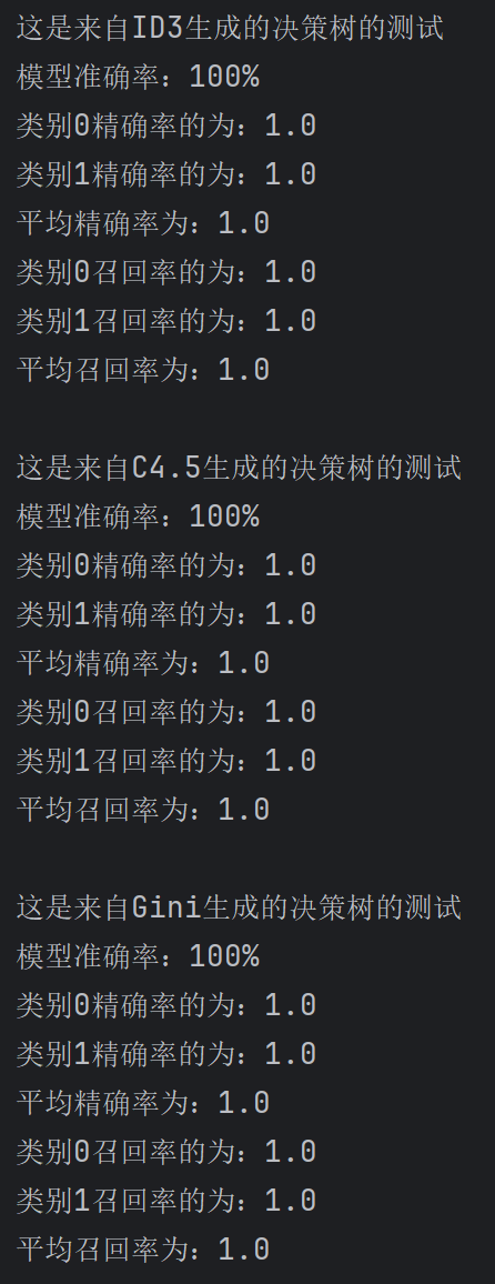
print(f"这是来自{func}生成的决策树的测试")
# 测试模型
accuracy = get_correct(dtree, test_features, test_tags)/test_features.shape[0]*100
precision, recallment = get_predict(dtree, test_features, test_tags, tags)
cf, queue = get_confusion(dtree, test_features, test_tags)
# 结果可视化
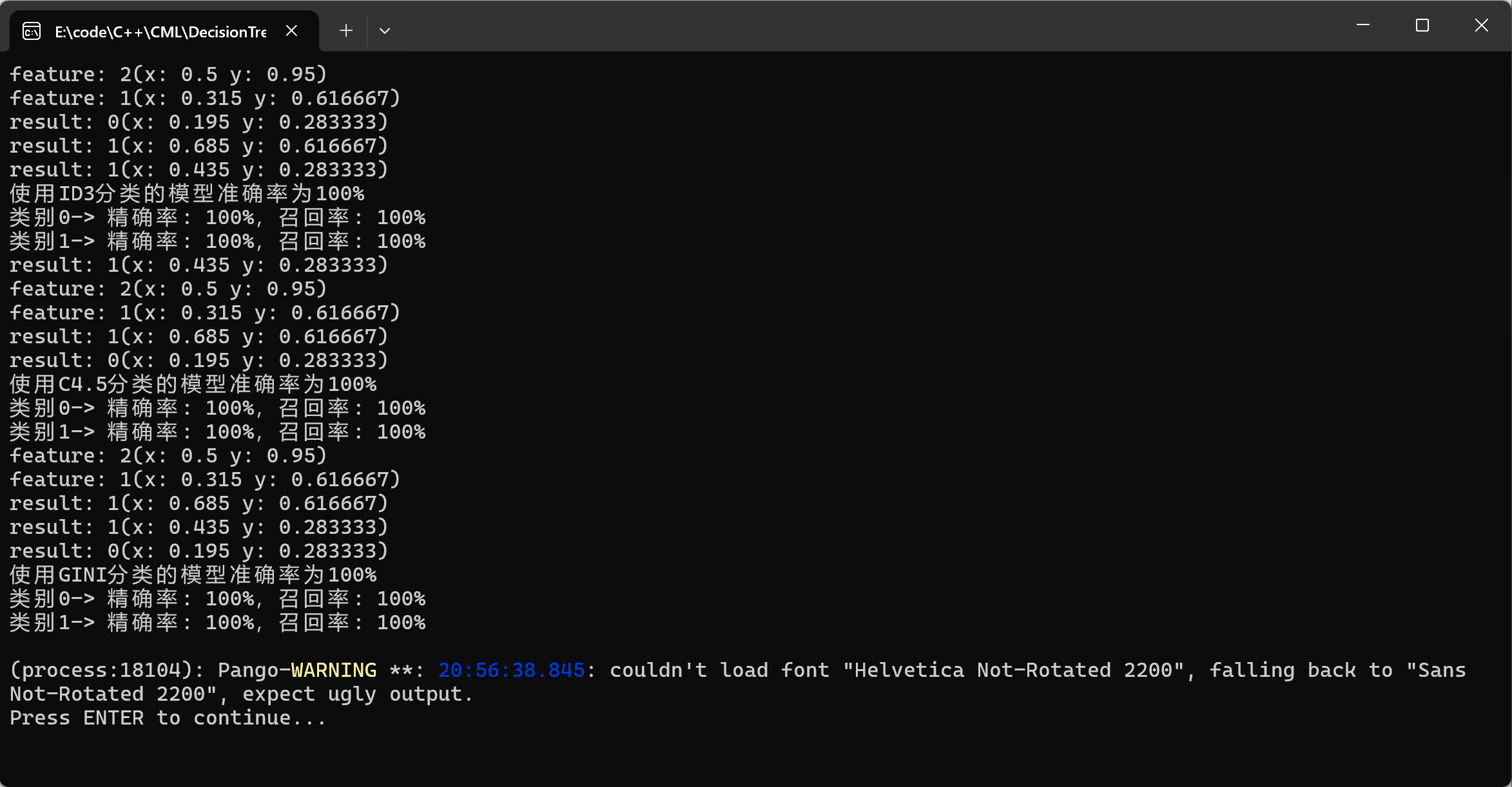
print(f"模型准确率:{accuracy:.0f}%")
print_dict(precision, "精确率")
print_dict(recallment, "召回率")
print()
# 决策树可视化
plot_decision_tree(dtree, max_level, axs[i, 0])
# 热力图可视化
plot_heatmap(cf, queue, axs[i, 1])
plt.tight_layout()
plt.show()3.2.3 核心代码讲解
算法思路和C++实现类似,前面的C++核心代码讲解基本都是在讲思路,这里就不重复了,一些语法的不同可以直接结合着代码看步骤。
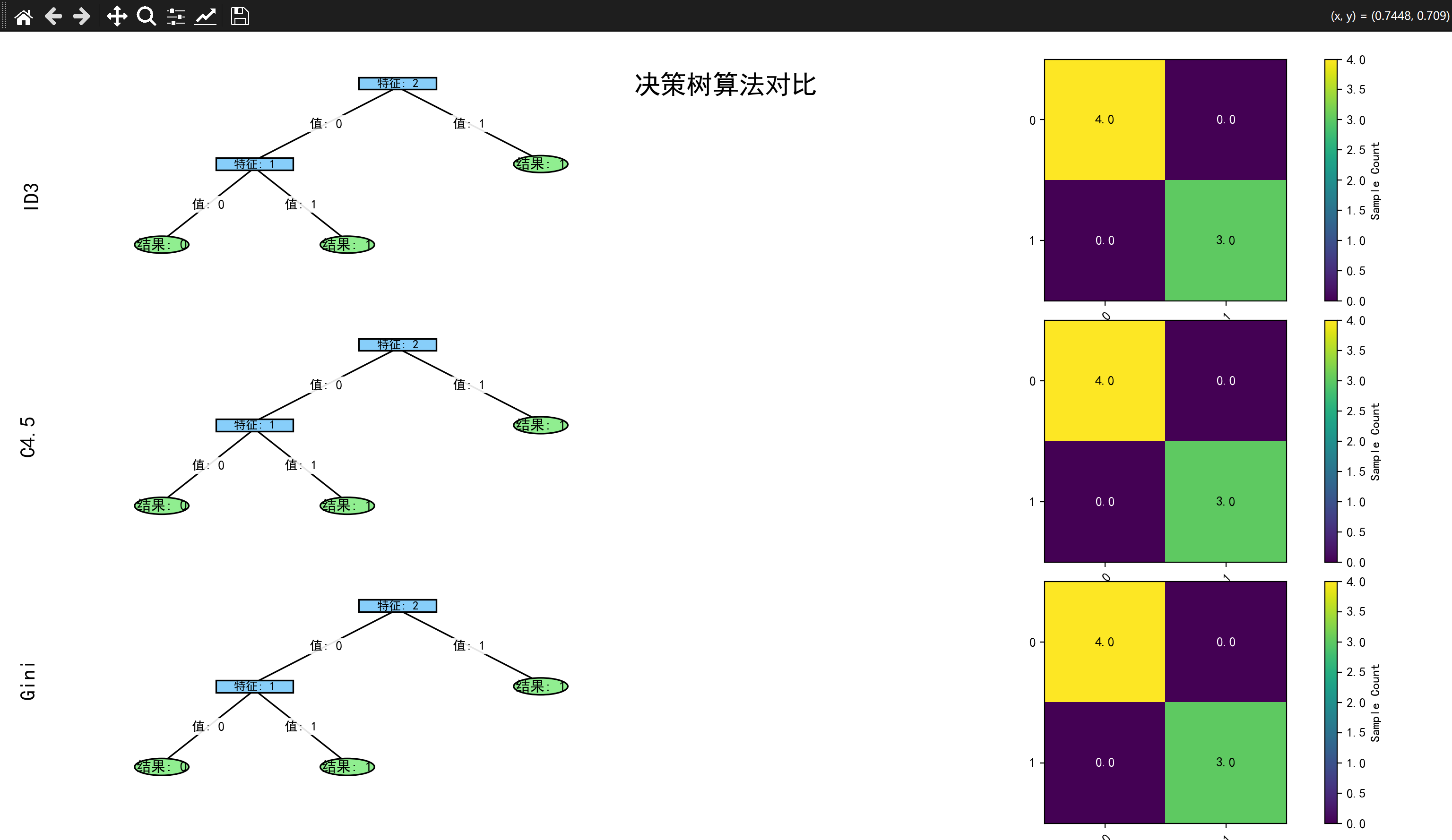
3.2.4 结果展示
四、总结
决策树是一个很符合人的直觉的一种模型,从结果上来看,拟合效果很高。
但是,拟合效果太高,会容易过拟合,所以我们需要对它进行剪枝,这里做一下下一篇博客的预告。