PyTorch实战（11）——随机连接神经网络（RandWireNN）

PyTorch实战（11）------随机连接神经网络（RandWireNN）

- [0. 前言](#0. 前言)
- [1. RandWireNN 原理](#1. RandWireNN 原理)
- [2. 使用 PyTorch 实现 RandWireNN](#2. 使用 PyTorch 实现 RandWireNN)
- - [2.1 定义训练函数](#2.1 定义训练函数)
  - [2.2 定义随机连接图](#2.2 定义随机连接图)
  - [2.3 定义 RandWireNN 模型模块](#2.3 定义 RandWireNN 模型模块)
  - [2.4 将随机图转化为神经网络](#2.4 将随机图转化为神经网络)
- [3. 训练 RandWireNN 模型](#3. 训练 RandWireNN 模型)
- [4. 评估和可视化 RandWireNN 模型](#4. 评估和可视化 RandWireNN 模型)
- 小结
- 系列链接

0. 前言

神经架构搜索 (Neural Architecture Search, NAS) 是深度学习一个热门领域，与面向特定任务的自动机器学习 (AutoML) 领域高度契合。AutoML 通过自动化数据集加载、架构设计和模型部署，显著降低了机器学习应用门槛。不同于传统人工设计网络结构，我们将实现一种通过架构生成器自动寻找最优拓扑的新型网络------随机连接神经网络 (RandWireNN)，RandWireNN 基于自动搜索最优架构的思想，通过随机图生成算法构建网络拓扑。在本节中，我们将探索 NAS，并使用 PyTorch 实现 RandWireNN 模型。

1. RandWireNN 原理

随机连接神经网络 (RandWireNN) 首先使用随机图生成算法来生成一个具有预定义节点数量的随机图，随后将该图通过一些定义被转化为神经网络：

有向性 (Directed)：图限制为有向图，边的方向表示神经网络中的数据流向
聚合机制 (Aggregation)：每个节点的多条输入边会通过可学习的加权求和进行特征聚合
转换操作 (Transformation)：每个节点内部执行标准操作组合：ReLU 激活→3×3 可分离卷积(常规 3×3 卷积接 1×1 逐点卷积)→批归一化，这个组合称为 ReLU-Conv-BN 三元组
分发机制 (Distribution)：从每个神经元发出的多条边都会携带三元组操作的副本

最后关键步骤是在图中添加唯一的输入节点(源)和输出节点(汇)，从而将随机图完整转化为神经网络架构。完成转化后，该网络即可用于各类机器学习任务的训练。

需要注意的是，出于可重复性考虑，ReLU-Conv-BN 三元组单元的输出通道数会保持与输入通道数一致。但实际应用中，可以根据任务需求，将多个通道数递增(同时数据/图像空间尺寸递减)的随机图级联起来，通过前一个图的汇节点与后一个图的源节点顺序连接。

接下来，使用 PyTorch 从零开始构建一个 RandWireNN 模型。

2. 使用 PyTorch 实现 RandWireNN

接下来，针对 CIFAR-10 图像分类任务开发 RandWireNN 模型。从一个空白模型开始，生成随机图，将其转化为神经网络，针对给定任务在指定数据集上训练，评估训练后的模型，并分析最终生成的模型结构。

2.1 定义训练函数

在本节中，我们将定义模型训练循环所需的训练函数，并创建数据集加载器来提供批训练数据。

(1) 首先，导入所需库：

python 复制代码

import torch
import torch.nn as nn
import torch.optim as optim
import torch.nn.functional as F
from torch.autograd import Variable
from torchvision import datasets, transforms
from torchviz import make_dot

import os
import time
import yaml
import random
import networkx as nx
import matplotlib.pyplot as plt

use_cuda = torch.cuda.is_available()
device = torch.device("cuda" if use_cuda else "cpu")

(2) 接下来，定义训练函数，该函数接收一个能对 RGB 输入图像生成预测概率的已训练模型：

python 复制代码

def set_lr(optim, epoch_num, lrate):
    lrate = lrate * (0.1 ** (epoch_num // 20))
    for params in optim.param_groups:
        params['lr'] = lrate

def train(model, train_dataloader, optim, loss_func, epoch_num, lrate):
    model.train()
    loop_iter = 0
    training_loss = 0
    training_accuracy = 0
    for training_data, training_label in train_dataloader:
        set_lr(optim, epoch_num, lrate)
        training_data, training_label = training_data.to(device), training_label.to(device)
        optim.zero_grad()
        pred_raw = model(training_data)
        curr_loss = loss_func(pred_raw, training_label)
        curr_loss.backward()
        optim.step()
        training_loss += curr_loss.data
        pred = pred_raw.data.max(1)[1]

        curr_accuracy = float(pred.eq(training_label.data).sum()) * 100. / len(training_data) 
        training_accuracy += curr_accuracy
        loop_iter += 1
        if loop_iter % 100 == 0:
            print(f"epoch {epoch_num}, loss: {curr_loss.data}, accuracy: {curr_accuracy}")

    data_size = len(train_dataloader.dataset) // batch_size
    return training_loss / data_size, training_accuracy / data_size

(3) 接下来，定义数据集加载器。使用经典的 CIFAR-10 数据集进行图像分类任务，该数据集包含 60000 张 32x32 的 RGB 图像，分为 10 个不同的类别，每个类别包含 6000 张图像。使用 torchvision.datasets 模块加载数据：

python 复制代码

def load_dataset(batch_size):
    transform_train_dataset = transforms.Compose([
        transforms.RandomCrop(32, padding=4),
        transforms.RandomHorizontalFlip(),
        transforms.ToTensor(),
        transforms.Normalize((0.4983, 0.4795, 0.4382), (0.2712, 0.2602, 0.2801)),
    ])

    transform_test_dataset = transforms.Compose([
        transforms.ToTensor(),
        transforms.Normalize((0.4983, 0.4795, 0.4382), (0.2712, 0.2602, 0.2801)),
    ])
    train_dataloader = torch.utils.data.DataLoader(
        datasets.CIFAR10('./data', transform=transform_train_dataset, train=True, download=True),
        batch_size=batch_size,
        shuffle=True
    )
    test_dataloader = torch.utils.data.DataLoader(
        datasets.CIFAR10('./data', transform=transform_test_dataset, train=False),
        batch_size=batch_size,
        shuffle=False
    )
    return train_dataloader, test_dataloader
train_dataloader, test_dataloader = load_dataset(batch_size)

接下来进入神经网络模型设计阶段，重点在于随机连接图的结构设计。

2.2 定义随机连接图

在本节中，我们将定义图生成器，用于生成随机图，后续将其转化为神经网络。

(1) 定义随机图生成器类：

python 复制代码

class RndGraph(object):
    def __init__(self, num_nodes, graph_probability, nearest_neighbour_k=4, num_edges_attach=5):
        self.num_nodes = num_nodes
        self.graph_probability = graph_probability
        self.nearest_neighbour_k = nearest_neighbour_k
        self.num_edges_attach = num_edges_attach

    def make_graph_obj(self):
        graph_obj = nx.random_graphs.connected_watts_strogatz_graph(self.num_nodes, self.nearest_neighbour_k, 
                                                                self.graph_probability)
        return graph_obj

在本节中，使用经典的随机图模型------Watts-Strogatz (WS) 模型，这也是 RandWireNN 原始论文中验证的三种图模型之一。该模型包含两个核心参数：

每个节点的邻居数 K K K (必须是偶数)
边重连概率 P P P

构建流程分为两步：

N N N 个节点环形排列，每个节点初始连接左右各 K / 2 K/2 K/2 个相邻节点
顺时针遍历每个节点 K / 2 K/2 K/2 次，在第 m m m 次遍历时 ( 0 < m < K / 2 0 < m < K/2 0<m<K/2)，以概率 P P P 重连当前节点与其右侧第 m m m 个邻居的边

其中，重连操作是指将该边替换为当前节点与除自身和第 m m m 个邻居外其他节点的连接。在代码实现中，图生成器类的 make_graph_obj 方法通过 networkx 库实例化 WS 图模型。

此外，我们还添加了 get_graph_config 方法来返回图中的节点和边的列表，便于后续转换为神经网络。我们还将定义一些图保存和加载方法，用于缓存生成的图，便于复现和提高效率：

python 复制代码

    def get_graph_config(self, graph_obj):
        incoming_edges = {}
        incoming_edges[0] = []
        node_list = [0]
        last = []
        for n in graph_obj.nodes():
            neighbor_list = list(graph_obj.neighbors(n))
            neighbor_list.sort()

            edge_list = []
            passed_list = []
            for nbr in neighbor_list:
                if n > nbr:
                    edge_list.append(nbr + 1)
                    passed_list.append(nbr)
            if not edge_list:
                edge_list.append(0)
            incoming_edges[n + 1] = edge_list
            if passed_list == neighbor_list:
                last.append(n + 1)
            node_list.append(n + 1)
        incoming_edges[self.num_nodes + 1] = last
        node_list.append(self.num_nodes + 1)
        return node_list, incoming_edges

    def save_graph(self, graph_obj, path_to_write):
        if not os.path.isdir("cached_graph_obj"):
            os.mkdir("cached_graph_obj")
        with open(f"./cached_graph_obj/{path_to_write}", "w") as fh:
            yaml.dump(graph_obj, fh)

    def load_graph(self, path_to_read):
        with open(f"./cached_graph_obj/{path_to_read}", "r") as fh:
            return yaml.load(fh, Loader=yaml.Loader)

接下来，开始创建实际的神经网络模型。

2.3 定义 RandWireNN 模型模块

完成图生成器后，我们需要将其转化为神经网络。首先设计以下基础模块用于转化过程。

(1) 可分离二维卷积层(底层模块)，可分离卷积层是由常规的 3x3 二维卷积层和一个逐点的 1x1 二维卷积层串联组成：

python 复制代码

class SepConv2d(nn.Module):
    def __init__(self, input_ch, output_ch, kernel_length=3, dilation_size=1, padding_size=1, stride_length=1, bias_flag=True):
        super(SepConv2d, self).__init__()
        self.conv_layer = nn.Conv2d(input_ch, input_ch, kernel_length, stride_length, padding_size, dilation_size, 
                              bias=bias_flag, groups=input_ch)
        self.pointwise_layer = nn.Conv2d(input_ch, output_ch, kernel_size=1, stride=1, padding=0, dilation=1, 
                                         groups=1, bias=bias_flag)

    def forward(self, x):
        return self.pointwise_layer(self.conv_layer(x))

(2) ReLU-Conv-BN 三元组单元：

python 复制代码

class UnitLayer(nn.Module):
    def __init__(self, input_ch, output_ch, stride_length=1):
        super(UnitLayer, self).__init__()

        self.dropout = 0.3

        self.unit_layer = nn.Sequential(
            nn.ReLU(),
            SepConv2d(input_ch, output_ch, stride_length=stride_length),
            nn.BatchNorm2d(output_ch),
            nn.Dropout(self.dropout)
        )

    def forward(self, x):
        return self.unit_layer(x)

作为核心变换单元，三元组单元是一个由 ReLU 层、可分离二维卷积层和批归一化 (Batch Normalization) 层串联而成的模块，此外还需要添加 Dropout 层用于正则化。

(3) 完成三元组单元的定义后，实现具有完整功能的图节点模块，包含前文所述的聚合、转换和分发功能：

python 复制代码

class GraphNode(nn.Module):
    def __init__(self, input_degree, input_ch, output_ch, stride_length=1):
        super(GraphNode, self).__init__()
        self.input_degree = input_degree
        if len(self.input_degree) > 1:
            self.params = nn.Parameter(torch.ones(len(self.input_degree), requires_grad=True))
        self.unit_layer = UnitLayer(input_ch, output_ch, stride_length=stride_length)

    def forward(self, *ip):
        if len(self.input_degree) > 1:
            op = (ip[0] * torch.sigmoid(self.params[0]))
            for idx in range(1, len(ip)):
                op += (ip[idx] * torch.sigmoid(self.params[idx]))
            return self.unit_layer(op)
        else:
            return self.unit_layer(ip[0])

在 forward 方法中，如果节点的输入边数量超过 1，当节点存在多条输入边时，系统会计算可学习权重的加权平均值。随后对该加权值应用三元组单元进行变换，最终输出经过转换 (ReLU-Conv-BN) 处理后的结果。

(4) 接下来，整合所有图和图节点的定义，构建完整的随机连接图类：

python 复制代码

class RandWireGraph(nn.Module):
    def __init__(self, num_nodes, graph_prob, input_ch, output_ch, train_mode, graph_name):
        super(RandWireGraph, self).__init__()
        self.num_nodes = num_nodes
        self.graph_prob = graph_prob
        self.input_ch = input_ch
        self.output_ch = output_ch
        self.train_mode = train_mode
        self.graph_name = graph_name

        rnd_graph_node = RndGraph(self.num_nodes, self.graph_prob)
        if self.train_mode is True:
            print("train_mode: ON")
            rnd_graph = rnd_graph_node.make_graph_obj()
            self.node_list, self.incoming_edge_list = rnd_graph_node.get_graph_config(rnd_graph)
            rnd_graph_node.save_graph(rnd_graph, graph_name)
        else:
            rnd_graph = rnd_graph_node.load_graph(graph_name)
            self.node_list, self.incoming_edge_list = rnd_graph_node.get_graph_config(rnd_graph)

        self.list_of_modules = nn.ModuleList([GraphNode(self.incoming_edge_list[0], self.input_ch, self.output_ch, 
                                                        stride_length=2)])
        self.list_of_modules.extend([GraphNode(self.incoming_edge_list[n], self.output_ch, self.output_ch) 
                                     for n in self.node_list if n > 0])

在该类的 __init__ 方法中，首先生成一个抽象的随机图，解析获取节点和边列表。使用 GraphNode 类，将每个抽象节点封装为神经网络神经元。最后，添加专用的源节点(输入)和汇节点(输出)以适配图像分类任务。

(5) 定义 forward 方法：

python 复制代码

    def forward(self, x):
        mem_dict = {}
        op = self.list_of_modules[0].forward(x)
        mem_dict[0] = op

        for n in range(1, len(self.node_list) - 1):
            if len(self.incoming_edge_list[n]) > 1:
                op = self.list_of_modules[n].forward(*[mem_dict[incoming_vtx] 
                                                       for incoming_vtx in self.incoming_edge_list[n]])
            else:
                op = self.list_of_modules[n].forward(mem_dict[self.incoming_edge_list[n][0]])
            mem_dict[n] = op
            
        op = mem_dict[self.incoming_edge_list[self.num_nodes + 1][0]]
        for incoming_vtx in range(1, len(self.incoming_edge_list[self.num_nodes + 1])):
            op += mem_dict[self.incoming_edge_list[self.num_nodes + 1][incoming_vtx]]
        return op / len(self.incoming_edge_list[self.num_nodes + 1])

首先，进行源神经元的前向传播，然后根据图的 list_of_nodes 对后续神经元进行一系列前向传播，每次前向传播使用 list_of_modules 执行。最后，通过汇节点的前向传播得到该图的输出。

接下来，基于这些预定义模块和随机连接图类构建完整的RandWireNN模型类。

2.4 将随机图转化为神经网络

在上一小节中，我们已经定义了单个随机连接图结构。然而，完整的随机连接神经网络应由多个级联的随机图组成。这样设计的核心理念在于：在图像分类任务中，随着网络从输入层向输出层推进，特征通道数应当逐步增加(同时空间尺寸逐步减小)。若仅使用单一随机图结构，由于设计约束，其特征通道数将保持恒定，无法实现这一需求。

(1) 首先定义完整的随机连接神经网络架构。该网络将包含三个随机连接图，这些图依次连接在一起，每个后续结构的通道数都是前一个的两倍，这符合图像分类任务中"通道递增、空间下采样"的通用设计准则：

python 复制代码

class RandWireNNModel(nn.Module):
    def __init__(self, num_nodes, graph_prob, input_ch, output_ch, train_mode):
        super(RandWireNNModel, self).__init__()
        self.num_nodes = num_nodes
        self.graph_prob = graph_prob
        self.input_ch = input_ch
        self.output_ch = output_ch
        self.train_mode = train_mode
        self.dropout = 0.3
        self.class_num = 10
            
        self.conv_layer_1 = nn.Sequential(
            nn.Conv2d(in_channels=3, out_channels=self.output_ch, kernel_size=3, padding=1),
            nn.BatchNorm2d(self.output_ch),
        )

        self.conv_layer_2 = nn.Sequential(
            RandWireGraph(self.num_nodes, self.graph_prob, self.input_ch, self.output_ch*2, self.train_mode, 
                          graph_name="conv_layer_2")
        )
        self.conv_layer_3 = nn.Sequential(
            RandWireGraph(self.num_nodes, self.graph_prob, self.input_ch*2, self.output_ch*4, self.train_mode, 
                          graph_name="conv_layer_3")
        )
        self.conv_layer_4 = nn.Sequential(
            RandWireGraph(self.num_nodes, self.graph_prob, self.input_ch*4, self.output_ch*8, self.train_mode, 
                          graph_name="conv_layer_4")
        )

        self.classifier_layer = nn.Sequential(
            nn.Conv2d(in_channels=self.input_ch*8, out_channels=1280, kernel_size=1),
            nn.BatchNorm2d(1280)
        )

        self.output_layer = nn.Sequential(
            nn.Dropout(self.dropout),
            nn.Linear(1280, self.class_num)
        )

__init__ 方法从一个常规的 3x3 卷积层开始，接着是通道数逐级倍增的随机连接图，然后是一个全连接层，将最后一个随机连接图最后一个神经元的卷积输出展平为一个 1280 维的向量。

(2) 最后，添加输出层，生成 10 维分类概率向量：

python 复制代码

    def forward(self, x):
        x = self.conv_layer_1(x)
        x = self.conv_layer_2(x)
        x = self.conv_layer_3(x)
        x = self.conv_layer_4(x)
        x = self.classifier_layer(x)

        # global average pooling
        _, _, h, w = x.size()
        x = F.avg_pool2d(x, kernel_size=[h, w])
        x = torch.squeeze(x)
        x = self.output_layer(x)

        return x

forward 方法在第一个全连接层之后应用了全局平均池化 (Global Average Pooling)，有助于减少网络的维度和参数数量。

我们已经成功定义了 RandWireNN 模型，加载了数据集，并定义了模型训练流程。接下来，运行模型训练循环。

3. 训练 RandWireNN 模型

在本节中，我们将设置模型的超参数并训练 RandWireNN 模型。

(1) 首先，声明必要的超参数：

python 复制代码

num_epochs = 5
graph_probability = 0.7
node_channel_count = 64
num_nodes = 16
lrate = 0.1
batch_size = 64
train_mode = True

(2) 定义辅助函数 plot_results：

python 复制代码

def plot_results(list_of_epochs, list_of_train_losses, list_of_train_accuracies, list_of_val_accuracies):
    plt.figure(figsize=(20, 9))
    plt.subplot(1, 2, 1)
    plt.plot(list_of_epochs, list_of_train_losses, label='training loss')
    plt.legend()

    plt.subplot(1, 2, 2)
    plt.plot(list_of_epochs, list_of_train_accuracies, label='training accuracy')
    plt.plot(list_of_epochs, list_of_val_accuracies, label='validation accuracy')
    plt.legend()
    if not os.path.isdir('./result_plots'):
        os.makedirs('./result_plots')
    plt.savefig('./result_plots/accuracy_plot_per_epoch.jpg')
    plt.close()

(3) 实例化 RandWireNN 模型，并设置优化器和损失函数：

python 复制代码

rand_wire_model = RandWireNNModel(num_nodes, graph_probability, node_channel_count, node_channel_count, train_mode).to(device)

optim_module = optim.SGD(rand_wire_model.parameters(), lr=lrate, weight_decay=1e-4, momentum=0.8)
loss_func = nn.CrossEntropyLoss().to(device)

(4) 启动训练循环：

python 复制代码

def accuracy(model, test_data_loader):
    model.eval()
    success = 0
    with torch.no_grad():
        for test_data, test_label in test_data_loader:
            test_data, test_label = test_data.to(device), test_label.to(device)
            pred_raw = model(test_data)
            pred = pred_raw.data.max(1)[1]
            success += pred.eq(test_label.data).sum()

    return float(success) * 100. / len(test_data_loader.dataset)
epochs = []
test_accuracies = []
training_accuracies = []
training_losses = []
best_test_accuracy = 0

start_time = time.time()
for ep in range(1, num_epochs + 1):
    epochs.append(ep)
    training_loss, training_accuracy = train(rand_wire_model, train_dataloader, optim_module, loss_func, ep, lrate)
    test_accuracy = accuracy(rand_wire_model, test_dataloader)
    test_accuracies.append(test_accuracy)
    training_losses.append(training_loss.item())
    training_accuracies.append(training_accuracy)
    print('test acc: {0:.2f}%, best test acc: {1:.2f}%'.format(test_accuracy, best_test_accuracy))

    if best_test_accuracy < test_accuracy:
        model_state = {
            'model': rand_wire_model.state_dict(),
            'accuracy': test_accuracy,
            'ep': ep,
        }
        if not os.path.isdir('model_checkpoint'):
            os.mkdir('model_checkpoint')
        model_filename = "ch_count_" + str(node_channel_count) + "_prob_" + str(graph_probability)
        torch.save(model_state, './model_checkpoint/' + model_filename + 'ckpt.t7')
        best_test_accuracy = test_accuracy
        plot_results(epochs, training_losses, training_accuracies, test_accuracies)
    print("model train time: ", time.time() - start_time)

输出结果如下所示：

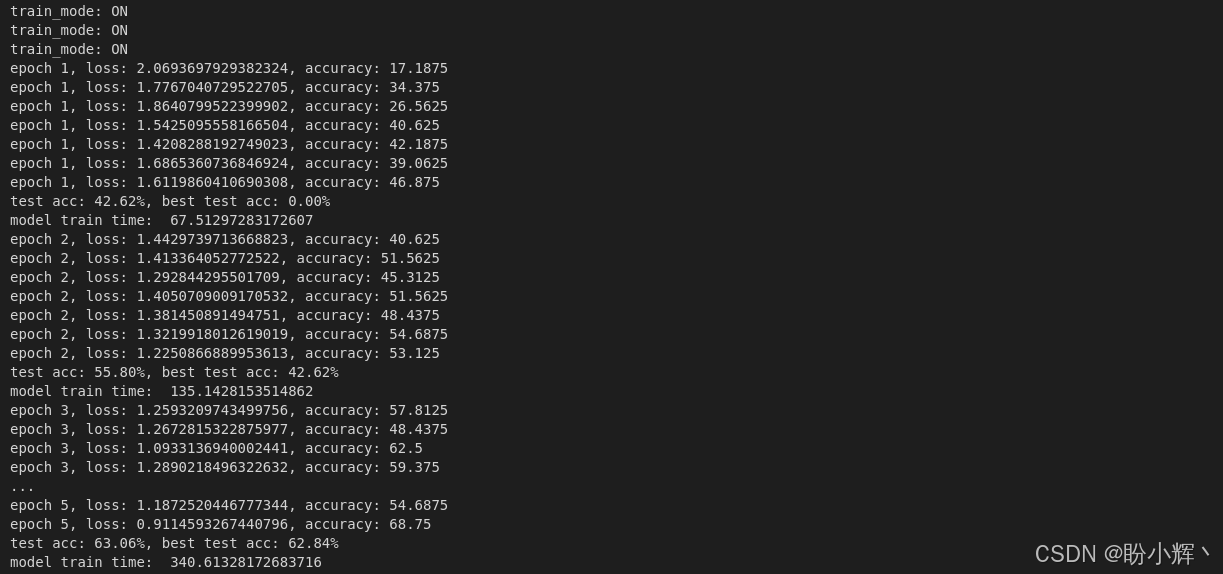
可以看到，随着训练进行，验证集上的准确率持续提升，表明模型具有良好的泛化能力。因此，可以说我们已经创建了一个没有特定架构的模型，它能够合理地执行 CIFAR-10 数据集上的图像分类任务。

4. 评估和可视化 RandWireNN 模型

最后，查看该模型在测试集上的表现，并从视觉上探索模型架构。

(1) 完成训练后，使用测试集进行评估：

python 复制代码

if os.path.exists("./model_checkpoint"):
    rand_wire_nn_model = RandWireNNModel(num_nodes, graph_probability, node_channel_count, node_channel_count, 
                                         train_mode=False).to(device)
    model_filename = "ch_count_" + str(node_channel_count) + "_prob_" + str(graph_probability)
    model_checkpoint = torch.load('./model_checkpoint/' + model_filename + 'ckpt.t7', weights_only=False)
    rand_wire_nn_model.load_state_dict(model_checkpoint['model'])
    last_ep = model_checkpoint['ep']
    best_model_accuracy = model_checkpoint['accuracy']
    print(f"best model accuracy: {best_model_accuracy}%, last epoch: {last_ep}")

    rand_wire_nn_model.eval()
    success = 0
    for test_data, test_label in test_dataloader:
        test_data, test_label = test_data.to(device), test_label.to(device)
        pred_raw = rand_wire_nn_model(test_data)
        pred = pred_raw.data.max(1)[1]
        success += pred.eq(test_label.data).sum()
    print(f"test accuracy: {float(success) * 100. / len(test_dataloader.dataset)} %")

else:
    assert False, "File not found. Please check again."

输出结果如下所示：

shell 复制代码

best model accuracy: 63.06%, last epoch: 5
test accuracy: 63.06 %

最佳模型出现在第 4 个训练epoch，测试准确率达到 63.06%。虽然仍有提升空间(可通过增加训练周期优化)，但相比随机猜测的 10% 基准准确率，这个由随机架构生成的网络已展现出令人满意的性能。

(2) 模型架构可视化：

python 复制代码

x = torch.randn(2, 3, 32, 32).to(device=device)
y = rand_wire_nn_model(x)
g = make_dot(y.mean(), params=dict(rand_wire_nn_model.named_parameters()))
g.format='svg'
g.filename = 'image2'
g.render(view=False)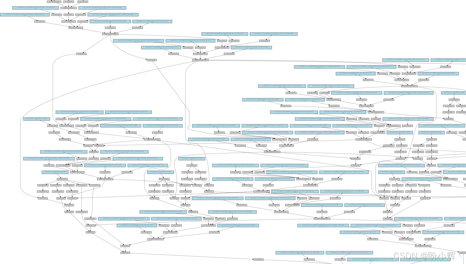

从上图中，可以观察到以下几个关键点：

起始阶段：包括一个 64 通道的 3x3 二维卷积层，后面接着一个 64 通道的 1x1 逐点二维卷积层
中间阶段：可以看到第三阶段随机图的汇点神经元 conv_layer_3 与第四阶段随机图的源点神经元 conv_layer_4 的衔接
输出阶段：第四阶段随机图的汇点神经元( 512 通道可分离二维卷积层)后接全连接层(生成 1280 维特征向量)，最终通过全连接 softmax 层输出 10 个类别的概率分布

至此，我们完成了一个特殊图像分类神经网络的构建、训练、测试与可视化------整个过程无需预设具体架构。虽然我们设定了部分约束条件(如 1280 维的倒数第二层特征向量长度、64 通道的可分离卷积层、4 阶段 RandWireNN 模型、ReLU-Conv-BN 三元组的神经元定义等)，但并未限定神经网络的具体连接结构，而是通过随机图生成器自动创建，这为探索最优架构提供了近乎无限的可能性。

小结

在本节中，我们探索了在固定参数优化之外进行架构优化的新思路------采用随机连接神经网络 (RandWireNN)，通过随机图生成、节点/边语义定义及子图互联构建神经网络，并使用 PyTorch 实现 RandWireNN 模型用于图像分类任务。

系列链接

PyTorch实战（1）------深度学习（Deep Learning）
PyTorch实战（2）------使用PyTorch构建神经网络
 PyTorch实战（3）------PyTorch vs. TensorFlow详解
 PyTorch实战（4）------卷积神经网络（Convolutional Neural Network，CNN）
PyTorch实战（5）------深度卷积神经网络
 PyTorch实战（6）------模型微调详解
 PyTorch实战（7）------循环神经网络
 PyTorch实战（8）------图像描述生成
 PyTorch实战（9）------从零开始实现Transformer
PyTorch实战（10）------从零开始实现GPT模型