@浙大疏锦行
今日任务:
- 通道注意力:模型的定义和插入的位置
- 通道注意力后的特征图和热力图
作业:对比不同卷积层热图可视化的结果
通道注意力
通道注意力是一种让网络能够自动学习每个特征通道重要性 的机制。它的核心思想:不同特征通道对当前任务的贡献不同,应该增强重要通道,抑制不重要通道。
# 伪代码:所有通道注意力的核心
def channel_attention(x):
    # 1. 计算每个通道的重要性权重
    channel_weights = compute_importance(x)  # 不同实现方式

    # 2. 对原始特征图进行通道级别加权
    output = x * channel_weights             # 相同的加权操作

return output其中,SE模块 是通道注意力实现 的一种具体方式 。SE模块包括三个核心操作:Squeeze (压缩)、Excitation (激励)、Scale(缩放)。
# SE 模块
输入 [B,C,H,W]
    ↓
Squeeze: 全局平均池化 → [B,C,1,1]
    ↓
Excitation: FC → ReLU → FC → Sigmoid → [B,C,1,1]
    ↓
Scale: 与输入逐通道相乘 → 输出 [B,C,H,W]
定义注意力模块
这里以SE模块的定义为例:
(1)Squeeze
- 通过全局平均池化 将每个通道的二维特征图(H×W)压缩为一个标量 ,保留通道的全局信息。
- 物理意义:计算每个通道在整个图像中的 "平均响应强度",例如,"边缘检测通道" 在有物体边缘的图像中响应值会更高。
python
# 全局平均池化
self.avg_pool = nn.AdaptiveAvgPool2d(1)
(2)Excitation
- 通过全连接层 + Sigmoid 激活 ,学习通道间的依赖关系,输出 0-1 之间的权重值。
- 物理意义:让模型自动判断哪些通道更重要 (权重接近 1),哪些通道可忽略(权重接近 0)。
python
# 全连接层 + Sigmoid激活
self.fc = nn.Sequential(
    nn.Linear(in_channel,in_channel//reduction_ratio,bias=False),
    nn.ReLU(inplace=True),
    nn.Linear(in_channel//reduction_ratio,in_channel,bias=False),
    nn.Sigmoid(),
    )
(3)Scale
- 将学习到的通道权重与原始特征图逐通道相乘,增强重要通道,抑制不重要通道。
- 物理意义:类似人类视觉系统聚焦于关键特征(如猫的轮廓),忽略无关特征(如背景颜色)
完整:
python
# SE模块的定义
class ChannelAttention(nn.Module):
    def __init__(self,in_channel,reduction_ratio=16):
        super(ChannelAttention,self).__init__()
        # 全局平均池化
        self.avg_pool = nn.AdaptiveAvgPool2d(1)
        # 全连接层 + Sigmoid激活
        self.fc = nn.Sequential(
            nn.Linear(in_channel,in_channel//reduction_ratio,bias=False),
            nn.ReLU(inplace=True),
            nn.Linear(in_channel//reduction_ratio,in_channel,bias=False),
            nn.Sigmoid(),
        )

    def forward(self,x):
        # 获得bath_size,channels等数值,为后续变换维度作准备
        batch_size,channels,height,width = x.size()

        # 1-squeeze
        avg_pool_out = self.avg_pool(x)

        # 展平为一维:[batch_size,channels],全连接层要求输入为一维
        avg_pool_out = avg_pool_out.view(batch_size,channels)
        # 2-获得通道权重
        channel_weights = self.fc(avg_pool_out)

        # 维度变换:匹配原始特征图的维度,[batch_size, channels, 1, 1]
        channel_weights = channel_weights.view(batch_size,channels,1,1)
        # 3-将权重应用到原始特征图上(逐通道相乘)
        return x*channel_weights # 输出形状:[batch_size, channels, height, width]
插入模型定义部分
在每一个卷积块中,插入SE模块:Conv → BN → ReLU → SE → Pool(常见顺序)。
- 信息完整:ReLU后的特征包含所有激活信息
- 池化前加权:在降采样前强调重要特征
python
# 在CNN架构中插入SE模块
class CNN(nn.Module):
def __init__(self):
super(CNN,self).__init__()
# ---------------------- 第一个卷积块 ----------------------
self.conv1 = nn.Conv2d(3,32,3,padding=1)
self.bn1 = nn.BatchNorm2d(32)
self.relu1 = nn.ReLU()
# 添加通道注意力
self.ca1 = ChannelAttention(in_channel=32,reduction_ratio=16)
self.pool1 = nn.MaxPool2d(2)
# ---------------------- 第二个卷积块 ----------------------
self.conv2 = nn.Conv2d(32,64,3,padding=1)
self.bn2 = nn.BatchNorm2d(64)
self.relu2 = nn.ReLU()
# 添加通道注意力
self.ca2 = ChannelAttention(in_channel=64,reduction_ratio=16)
self.pool2 = nn.MaxPool2d(2)
# ---------------------- 第三个卷积块 ----------------------
self.conv3 = nn.Conv2d(64,128,3,padding=1)
self.bn3 = nn.BatchNorm2d(128)
self.relu3 = nn.ReLU()
# 添加通道注意力
self.ca3 = ChannelAttention(in_channel=128,reduction_ratio=16)
self.pool3 = nn.MaxPool2d(2)
# ---------------------- 全连接器 ----------------------
self.fc1 = nn.Linear(128*4*4,512)
self.dropout = nn.Dropout(p=0.5)
self.fc2 = nn.Linear(512,10)
def forward(self,x):
# ---------- 卷积块1处理 ----------
x = self.conv1(x)
x = self.bn1(x)
x = self.relu1(x)
x = self.ca1(x) # 应用通道注意力
x = self.pool1(x)
# ---------- 卷积块2处理 ----------
x = self.conv2(x)
x = self.bn2(x)
x = self.relu2(x)
x = self.ca2(x) # 应用通道注意力
x = self.pool2(x)
# ---------- 卷积块3处理 ----------
x = self.conv3(x)
x = self.bn3(x)
x = self.relu3(x)
x = self.ca3(x) # 应用通道注意力
x = self.pool3(x)
# ---------- 展平与全连接层 ----------
x = x.view(-1, 128 * 4 * 4)
x = self.fc1(x)
x = self.relu3(x)
x = self.dropout(x)
x = self.fc2(x)
return x
# 实例化
model = CNN().to(device)
# 损失函数、优化器、学习率调度器
criterion = nn.CrossEntropyLoss()
optimizer = optim.Adam(model.parameters(),lr=0.001)
scheduler = optim.lr_scheduler.ReduceLROnPlateau(optimizer,mode='min',factor=0.5,patience=3)
# 训练模型(复用原有的train函数)
print("开始训练带通道注意力的CNN模型...")
final_accuracy = train(model, train_loader, test_loader, criterion, optimizer, scheduler, device, epochs=50)
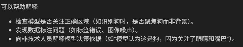
print(f"训练完成!最终测试准确率: {final_accuracy:.2f}%")可视化空间注意力热图
整体的思路与特征图可视化是类似的,这里选择对最后一个卷积层可视化。
步骤
(1)初始化设置
python
# 1-初始化设置
model.eval()
class_names = ['airplane', 'automobile', 'bird', 'cat', 'deer', 'dog', 'frog', 'horse', 'ship', 'truck']
(2)数据加载与处理
python
# 2-数据加载与处理
for i,(images,labels) in enumerate(test_loader):
    if i >= num_samples:
        break
    images,labels = images.to(device),labels.to(device)
(3)注册钩子捕获特征图
python
# 3-注册钩子捕获特征图
activation_maps = []
# 定义钩子
def hook(module,input,output):
    activation_maps.append(output.cpu())

forward_hook = model.conv3.register_forward_hook(hook)
(4)前向传播与特征提取
python
# 4-前向传播与特征提取
output = model(images) # 前向传播,触发钩子
forward_hook.remove() # 移除钩子
_,predicted = torch.max(output,1) # 获取预测结果
(5)可视化热图
这里需要计算通道注意力权重,然后选取前n个活跃通道(权重大)可视化。
- 通道归一化:保证颜色映射的一致性
- 尺寸匹配:热力图与原始图像尺寸要匹配
- 图像叠加:原始图像作为底图,热力图叠加
python
# 5-可视化热图
# 反标准化--原始图像
img = images[0].cpu().permute(1,2,0).numpy()
img = img * np.array([0.2023, 0.1994, 0.2010]).reshape(1, 1, 3) + np.array([0.4914, 0.4822, 0.4465]).reshape(1, 1, 3)
img = np.clip(img, 0, 1)
# 获取激活图(最后一个卷积层的输出)
feature_maps = activation_maps[0][0].cpu() # 获取第一个样本, [C, H, W]
channel_weights = torch.mean(feature_maps,dim=(1,2))
sorted_weight = torch.argsort(channel_weights,descending=True)
# 创建子图
fig,axes = plt.subplots(1,4,figsize=(16,4))
# 绘制原始图像
axes[0].imshow(img)
axes[0].set_title(f'Original Picture\nActual:{class_names[labels[0]]}\nPredicted:{class_names[predicted[0]]}')
axes[0].axis('off')
for j in range(3):
channel_idx = sorted_weight[j] # 获得通道索引
channel_map = feature_maps[channel_idx].numpy() # 获得单通道,[H, W]
# 归一化
channel_map = (channel_map - channel_map.min()) / (channel_map.max() - channel_map.min()+1e-8)
# 调整热图大小,匹配原始图像
from scipy.ndimage import zoom
heatmap = zoom(channel_map,(32/feature_maps.shape[1],32/feature_maps.shape[2]))
# 叠加图像
axes[j+1].imshow(img)
axes[j+1].imshow(heatmap,alpha=0.5,cmap='jet')
axes[j+1].set_title(f'Attention Heatmap - Channnel {channel_idx}')
axes[j+1].axis('off')
plt.tight_layout()
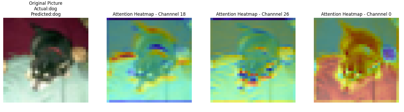
plt.show()结果
python
# 注意力热图可视化
def visualize_attention_map(model,test_loader,device,num_samples=3):
# 1-初始化设置
model.eval()
class_names = ['airplane', 'automobile', 'bird', 'cat', 'deer', 'dog', 'frog', 'horse', 'ship', 'truck']
with torch.no_grad():
# 2-数据加载与处理
for i,(images,labels) in enumerate(test_loader):
if i >= num_samples:
break
images,labels = images.to(device),labels.to(device)
# 3-注册钩子捕获特征图
activation_maps = []
# 定义钩子
def hook(module,input,output):
activation_maps.append(output.cpu())
forward_hook = model.conv3.register_forward_hook(hook)
# 4-前向传播与特征提取
output = model(images) # 前向传播,触发钩子
forward_hook.remove() # 移除钩子
_,predicted = torch.max(output,1) # 获取预测结果
# 5-可视化热图
# 反标准化--原始图像
img = images[0].cpu().permute(1,2,0).numpy()
img = img * np.array([0.2023, 0.1994, 0.2010]).reshape(1, 1, 3) + np.array([0.4914, 0.4822, 0.4465]).reshape(1, 1, 3)
img = np.clip(img, 0, 1)
# 获取激活图(最后一个卷积层的输出)
feature_maps = activation_maps[0][0].cpu() # 获取第一个样本, [C, H, W]
channel_weights = torch.mean(feature_maps,dim=(1,2))
sorted_weight = torch.argsort(channel_weights,descending=True)
# 创建子图
fig,axes = plt.subplots(1,4,figsize=(16,4))
# 绘制原始图像
axes[0].imshow(img)
axes[0].set_title(f'Original Picture\nActual:{class_names[labels[0]]}\nPredicted:{class_names[predicted[0]]}')
axes[0].axis('off')
for j in range(3):
channel_idx = sorted_weight[j] # 获得通道索引
channel_map = feature_maps[channel_idx].numpy() # 获得单通道,[H, W]
# 归一化
channel_map = (channel_map - channel_map.min()) / (channel_map.max() - channel_map.min()+1e-8)
# 调整热图大小,匹配原始图像
from scipy.ndimage import zoom
heatmap = zoom(channel_map,(32/feature_maps.shape[1],32/feature_maps.shape[2]))
# 叠加图像
axes[j+1].imshow(img)
axes[j+1].imshow(heatmap,alpha=0.5,cmap='jet')
axes[j+1].set_title(f'Attention Heatmap - Channnel {channel_idx}')
axes[j+1].axis('off')
plt.tight_layout()
plt.show()
# 调用可视化函数
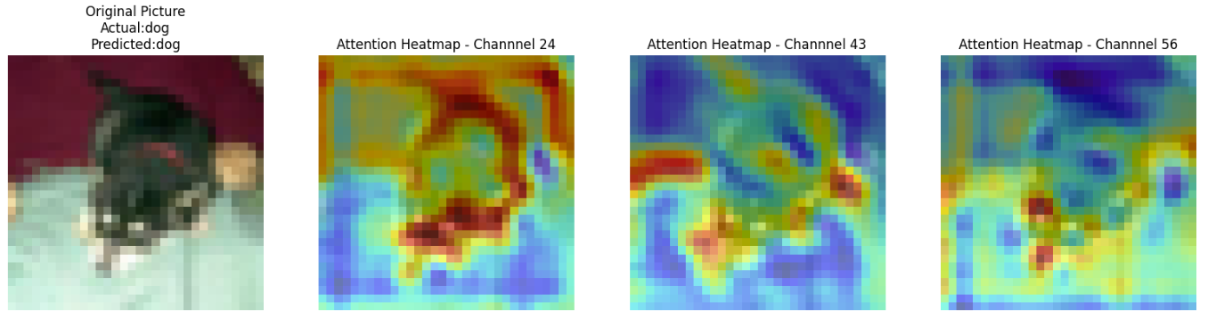
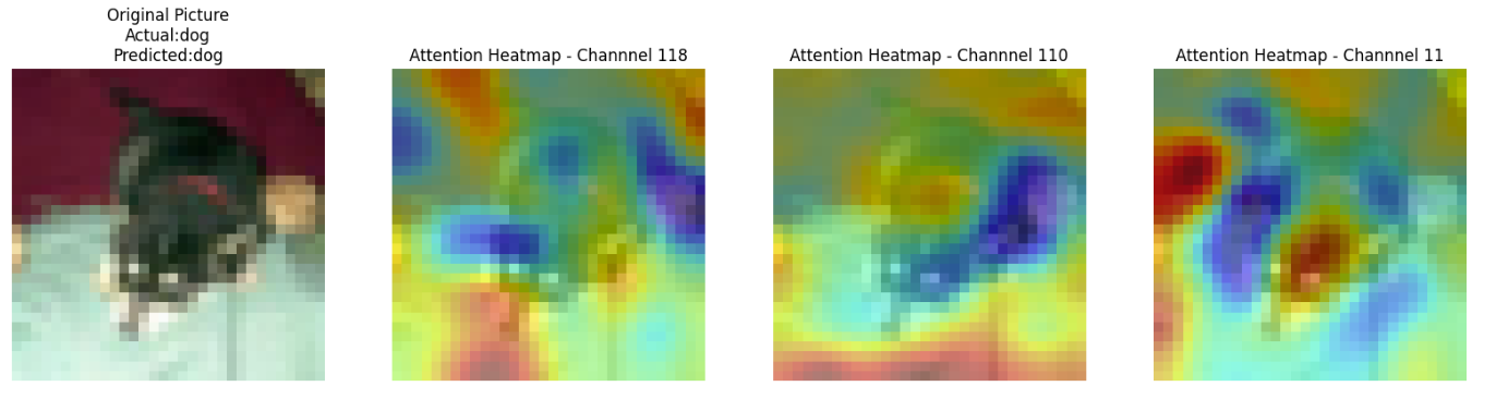
visualize_attention_map(model, test_loader, device, num_samples=3)未加入通道注意力的版本:
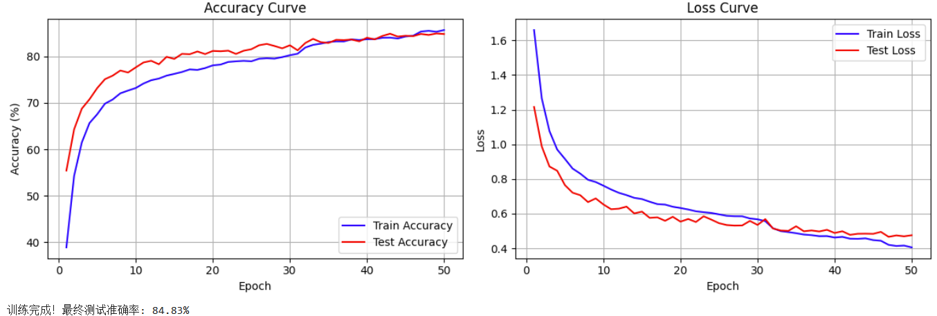
加入通道注意力的版本:
作业
修改注册钩子的模块,改成conv1和conv2:
python
forward_hook = model.conv3.register_forward_hook(hook)conv1(第一层卷积)
conv2(第二层卷积)
conv3(第三层卷积)
小结
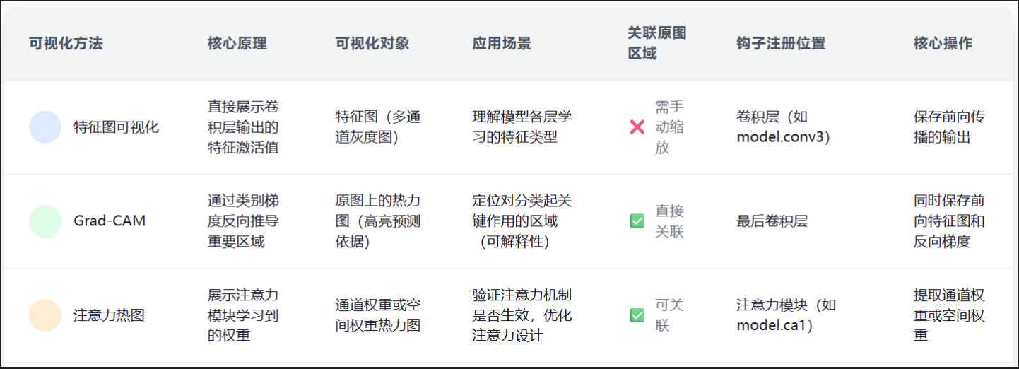
(1)热图分析:红色表示高关注(对分类最重要的区域),蓝色表示低关注。如果热力图错误聚焦(红色区域)在背景上,可能说明模型过拟合或训练不足。
(2)多通道对比:不同的通道关注不同的特征,比如整体轮廓、纹理细节、颜色分布。
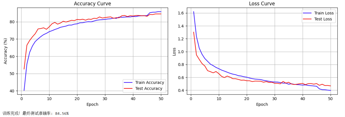
(3)使用热图可视化的应用: