目录
[Steady-State Analysis of a Linear Circuit](#Steady-State Analysis of a Linear Circuit)
[Transient Analysis of a Linear Circuit](#Transient Analysis of a Linear Circuit)
[向量仿真phasor simulation](#向量仿真phasor simulation)
前言
本次拆解了两个模型分别是:Steady-State Analysis of a Linear Circuit和Transient Analysis of a Linear Circuit。可在官方文档搜索对应模型或找到对应文件夹打开。
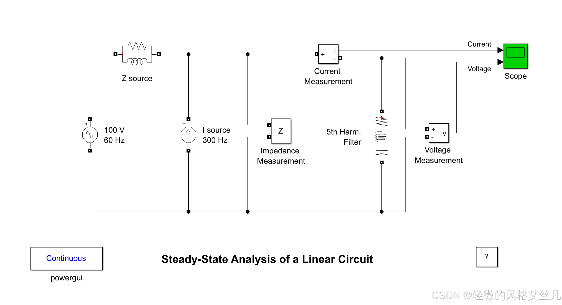
Steady-State Analysis of a Linear Circuit
官方说明
Description
A 5th harmonic filter is connected at a bus bar fed by a 60 Hz, 100 V inductive source. A 5th harmonic (300 Hz, 1 A) current is injected at the bus bar.
This linear system consists of 3 states (2 inductor currents and 1 capacitor voltage), 2 inputs (Vs, Is) and 2 outputs (Current and Voltage Measurement).
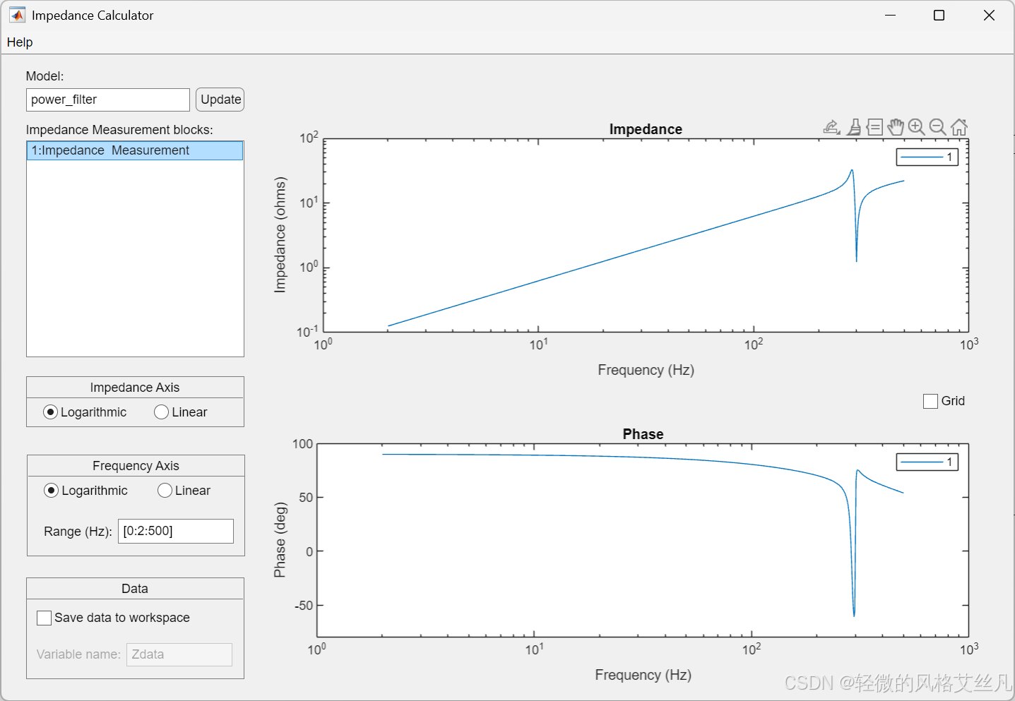
An Impedance Measurement block is used to compute the impedance versus frequency of the circuit.
Simulation
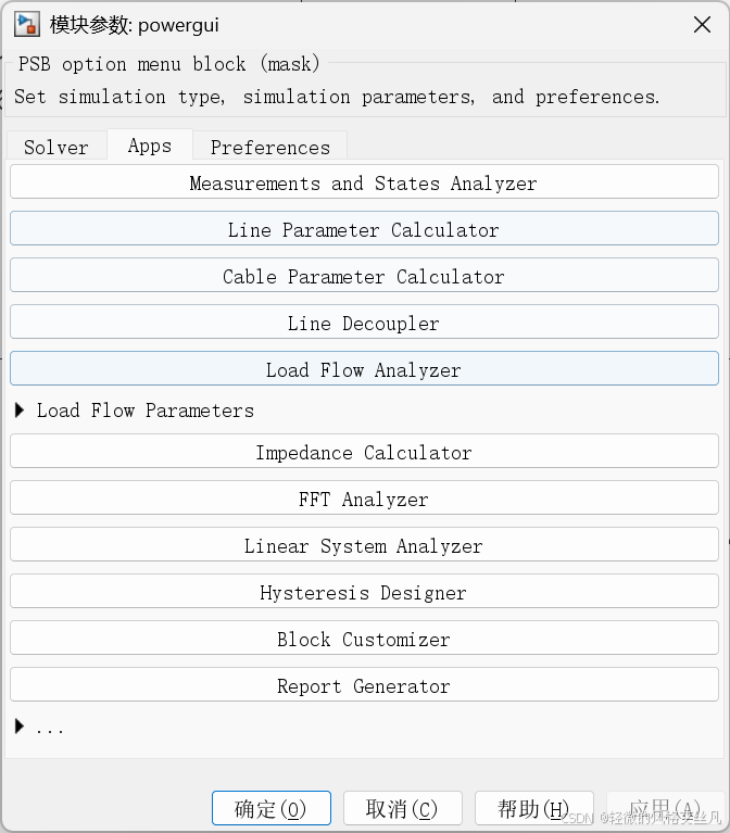
Use the Powergui block to find the steady-state 60Hz and 300 Hz components of voltage and current phasors. The values of the 3 states (phasors and initial values) can be also obtained from the powergui block.
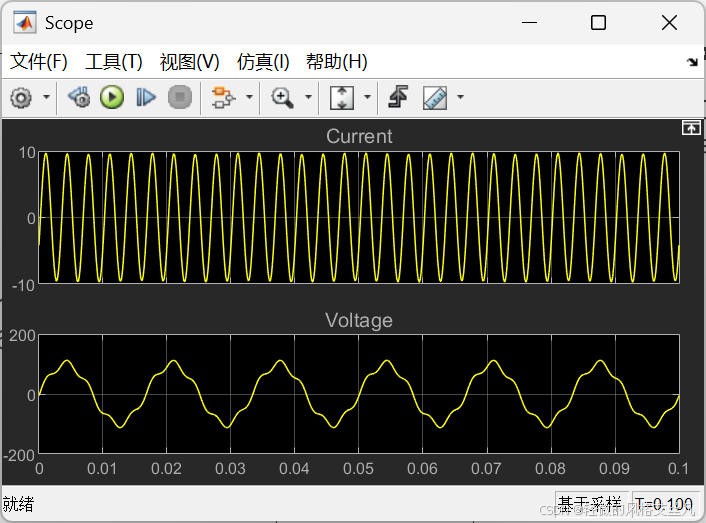
Open the scope and start the simulation from the Simulation/Start menu. Notice that the simulation starts in steady-state. Using the Powergui block, select Impedance vs Frequency Measurement. A new window opens.
The measurement will be performed for the specified frequency range vector 0: 2:1000 (0 to 1000 Hz by steps of 2 Hz). Click on the Display button. The impedance is displayed in a graphic window. Notice the series resonance at 300 Hz corresponding to the tuned frequency of the filter.
描述
在由 60 赫兹、100 伏感性电源供电的母线上,连接了一个 5 次谐波滤波器。向该母线注入 5 次谐波(300 赫兹、1 安)电流。
该线性系统包含 3 个状态量(2 个电感电流和 1 个电容电压)、2 个输入量(电源电压 Vs、注入电流 Is)以及 2 个输出量(电流测量值和电压测量值)。
系统中采用阻抗测量模块,用于计算电路阻抗随频率的变化关系。
仿真步骤
- 使用 Powergui 模块获取 60 赫兹和 300 赫兹下电压与电流相量的稳态分量。3 个状态量(相量及初始值)也可通过该模块获取。
- 打开示波器,从 "仿真(Simulation)/ 启动(Start)" 菜单启动仿真。需注意,仿真将从稳态开始。通过 Powergui 模块选择 "阻抗 - 频率测量(Impedance vs Frequency Measurement)",将弹出一个新窗口。
- 测量将在指定的频率范围向量 0: 2:1000(即从 0 赫兹到 1000 赫兹,步长为 2 赫兹)内进行。点击 "显示(Display)" 按钮,阻抗曲线将在图形窗口中显示。需注意,在 300 赫兹处会出现串联谐振,该频率与滤波器的调谐频率一致。
试运行
验算
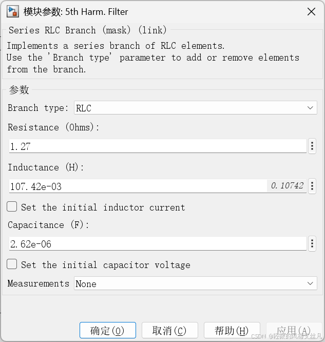
要计算该串联 RLC 支路的谐振频率,需使用串联谐振频率公式:f0=2πLC1
代入参数(从模块参数中获取):
- 电感 L=107.42e−3 H=0.10742 H
- 电容 C=2.62e−6 F
计算过程:
先计算 LC:LC=0.10742×2.62e−6≈2.8144e−7LC≈2.8144e−7≈5.305e−4
代入谐振频率公式:f0=2×π×5.305e−41≈3.332e−31≈300 Hz
最终该 RLC 支路的谐振频率约为 300Hz(与之前描述的 "5 次谐波滤波器调谐频率" 一致)。
Transient Analysis of a Linear Circuit
官方说明
Description
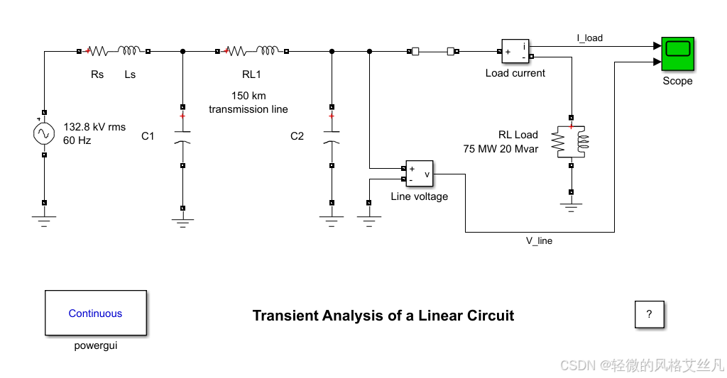
This circuit is a simplified model of a 230 kV three-phase power system. Only one phase of the transmission system is represented. The equivalent source is modeled by a voltage source (230 kV rms/sqrt(3) or 187.8 kV peak, 60 Hz) in series with its internal impedance (Rs Ls) corresponding to a 3-phase 2000 MVA short circuit level and X/R = 10. (X = 230e3^2/2000e6 = 26.45 ohms or L = 0.0702 H, R = X/10 = 2.645 ohms). The source feeds a RL load through a 150 km transmission line. The line distributed parameters (R = 0.035ohm/km, L = 0.92 mH/km, C = 12.9 nF/km) are modeled by a single pi section (RL1 branch 5.2 ohm; 138 mH and two shunt capacitances C1 and C2 of 0.967 uF). The load (75 MW - 20 Mvar per phase) is modeled by a parallel RLC load block.
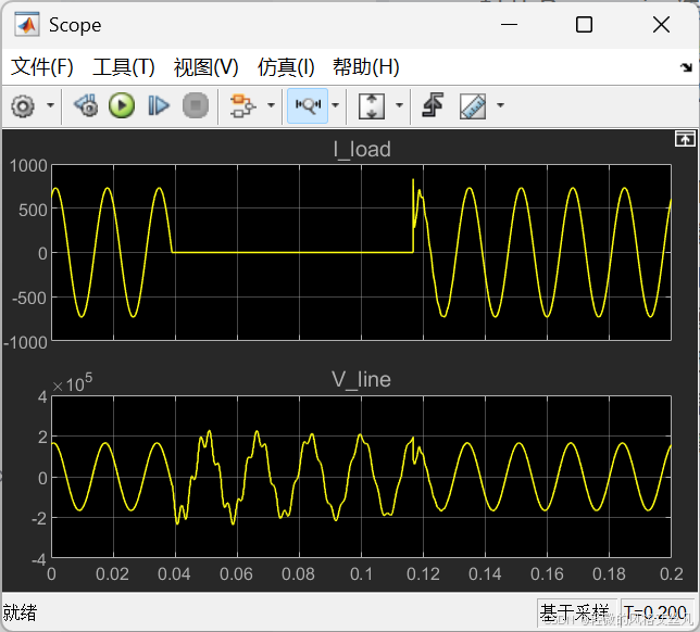
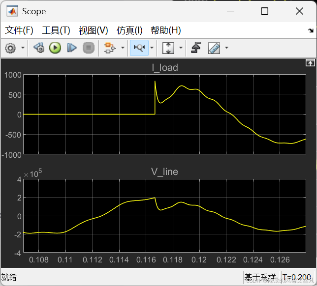
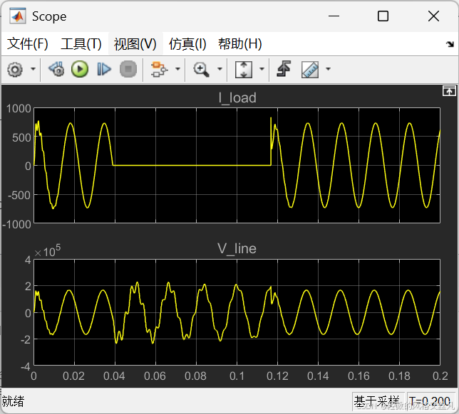
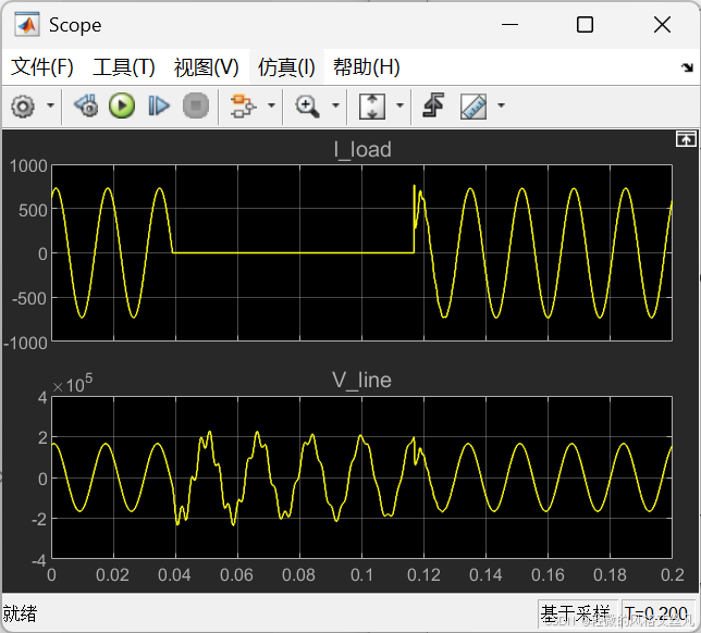
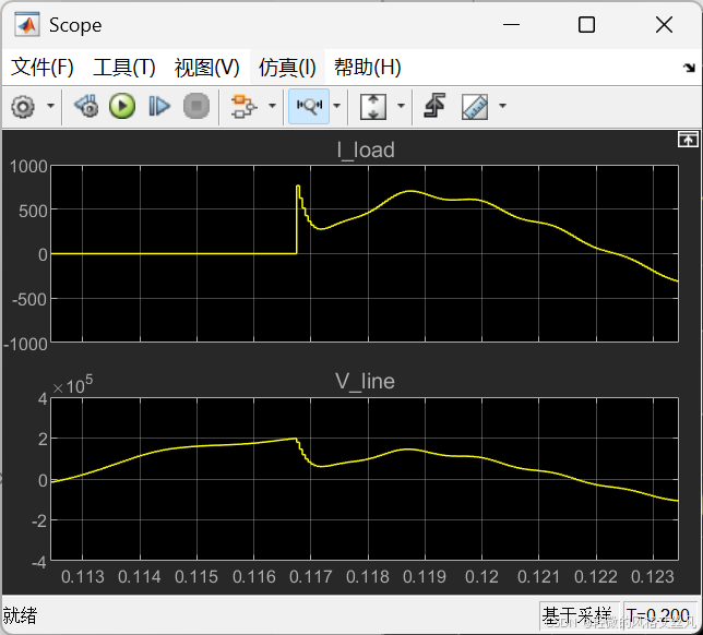
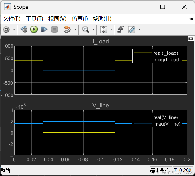
A circuit breaker is used to switch the load at the receiving end of the transmission line. The breaker which is initially closed is opened at t = 2 cycles, then it is reclosed at t = 7 cycles. Current and Voltage Measurement blocks provide signals for visualization purpose.
Simulation
1. Simulation using a continuous solver (ode23tb)
Start the simulation and observe line voltage and load current transients during load switching and note that the simulation starts in steady-state. Use the zoom buttons of the oscilloscope to observe the transient voltage at breaker reclosing.
2. Using the Powergui to obtain steady-state phasors and set initial states
Open the Powergui block and select "Steady State Voltage and Currents" to measure the steady-state voltage and current phasors. Using the Powergui select now "Initial States Setting" to obtain the initial state values (voltage across capacitors and current in inductances). Now, reset all the initial states to zero by clicking the "to zero" button and then "Apply" to confirm changes. Restart the simulation and observe transients at simulation starting. Using the same Powergui window, you can also set selected states to specific values.
3. Discretizing your circuit and simulating at fixed steps
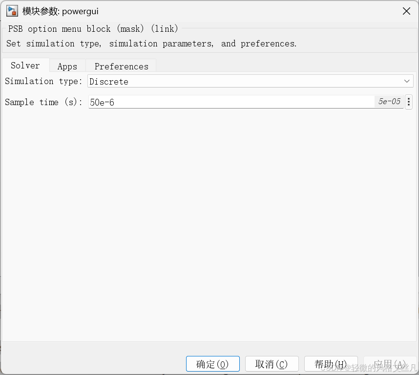
The Powergui block can also be used to discretize your circuit and simulate it at fixed steps. Open the Powergui. Select "Discretize electrical model" and specify a sample time of 50e-6 s. The state-space model will now be discretized using trapezoidal fixed step integration. The precision of results is now imposed by the sample time. Restart the simulation and compare simulation results with the continuous integration method. Vary the sample time of the discrete system and note the impact on precision of fast transients.
4. Using the phasor simulation method
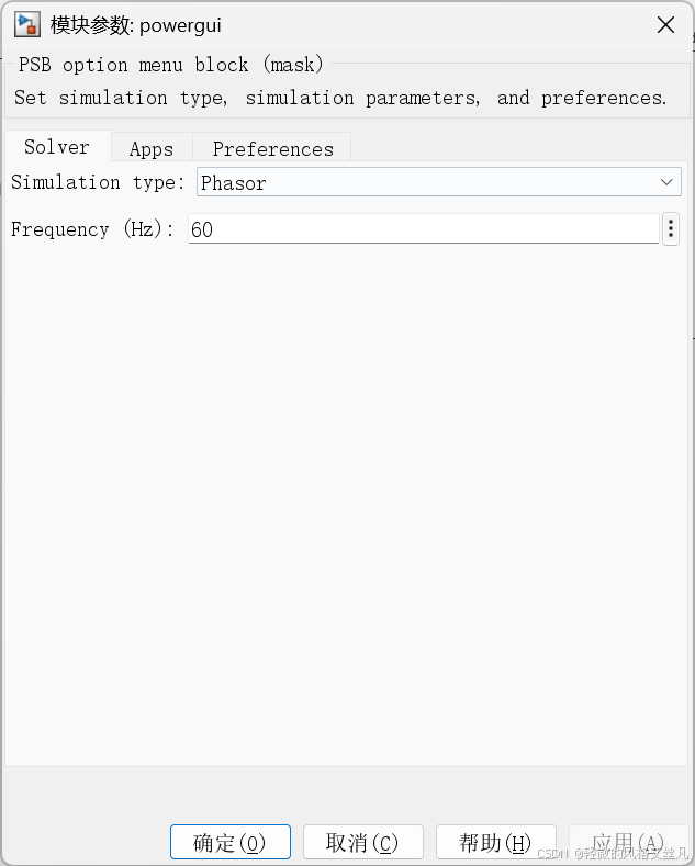
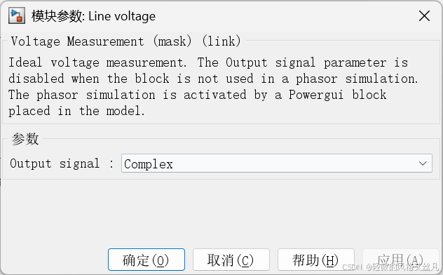
You will now use a third simulation technique. The "phasor simulation" method consists to replace the circuit state-space model by a set of algebraic equations evaluated at a fixed frequency and to replace sinusoidal voltage and current sources by phasors (complex numbers). This method allows a fast computation of voltage and current phasors at a selected frequency, disregarding fast transients. It is particularly efficient to study electromechanical transients of generators and motors involving low frequency oscillation modes. Open the Powergui block and select "Phasor simulation". Restart the simulation. Observe that the magnitude of 60 Hz voltage and current is now displayed on the scope. If you double click on the voltage or current measurement block you can choose to output phasor signals in four different formats: Complex, Real/Imag, Magnitude/Angle (in degrees), or just Magnitude (default value). Notice that you cannot send a complex signal to an oscilloscope.
描述
该电路是 230 千伏三相电力系统的简化模型,仅展示了输电系统的一相。等效电源由一个电压源(有效值为 230 千伏 /√3,峰值为 187.8 千伏,频率 60 赫兹)与其内阻(Rs、Ls)串联构成,对应三相短路容量 2000 兆伏安、X/R=10 的参数(电抗 X=230e3²/2000e6=26.45 欧姆,即电感 L=0.0702 亨利;电阻 R=X/10=2.645 欧姆)。电源通过一条 150 千米的输电线路向 RL 负载供电。线路的分布参数(电阻 0.035 欧姆 / 千米、电感 0.92 毫亨 / 千米、电容 12.9 纳法 / 千米)由单个 π 型等效电路建模(RL1 支路:5.2 欧姆、138 毫亨;两个并联电容 C1 和 C2,各 0.967 微法)。负载(每相 75 兆瓦、20 兆乏)由并联 RLC 负载模块建模。
输电线路受电端采用断路器控制负载通断:断路器初始处于闭合状态,在 t=2 个周期时断开,随后在 t=7 个周期时重合闸。电流和电压测量模块用于提供可视化信号。
仿真步骤
使用连续求解器(ode23tb)仿真启动仿真,观察负载投切过程中的线路电压和负载电流暂态过程,注意仿真从稳态开始。利用示波器的缩放按钮,观察断路器重合闸时的暂态电压。
通过 Powergui 获取稳态相量并设置初始状态打开 Powergui 模块,选择 "稳态电压和电流" 以测量稳态电压和电流相量。再通过 Powergui 选择 "初始状态设置",获取初始状态值(电容电压、电感电流)。点击 "置零" 按钮将所有初始状态重置为零,再点击 "应用" 确认修改。重新启动仿真,观察仿真启动时的暂态过程。通过同一 Powergui 窗口,也可将特定状态设置为指定值。
离散化电路并以固定步长仿真Powergui 模块也可用于离散化电路并以固定步长仿真。打开 Powergui,选择 "离散化电气模型" 并指定采样时间为 50e-6 秒。状态空间模型将通过梯形固定步长积分法离散化,结果精度由采样时间决定。重新启动仿真,将结果与连续积分法的结果对比。调整离散系统的采样时间,观察其对快速暂态过程精度的影响。
使用相量仿真法接下来使用第三种仿真技术:"相量仿真" 法会将电路状态空间模型替换为固定频率下的代数方程组,并将正弦电压、电流源替换为相量(复数)。该方法可快速计算选定频率下的电压、电流相量,忽略快速暂态过程,尤其适用于研究发电机、电动机涉及低频振荡模式的机电暂态过程。打开 Powergui 模块,选择 "相量仿真",重新启动仿真。观察示波器上显示的 60 赫兹电压、电流的幅值。双击电压或电流测量模块,可选择将相量信号以四种格式输出:复数、实部 / 虚部、幅值 / 角度(单位:度),或仅幅值(默认值)。需注意,无法将复信号直接发送至示波器。
试运行
示波器
稳态与初始化
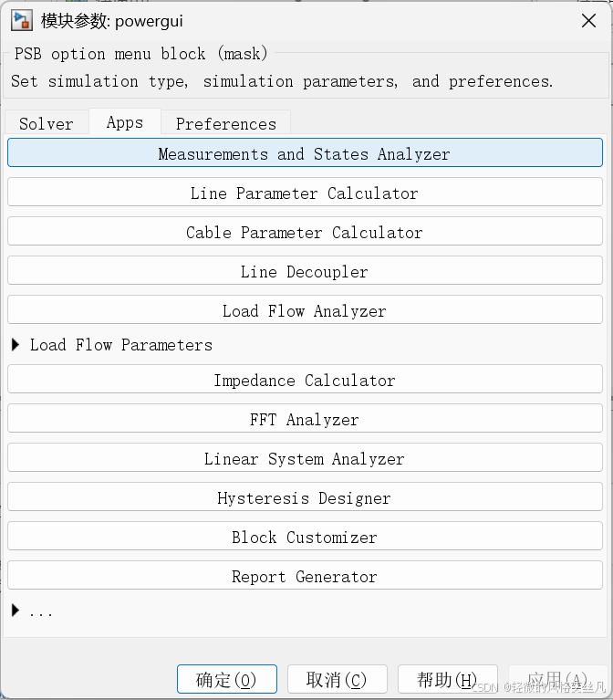
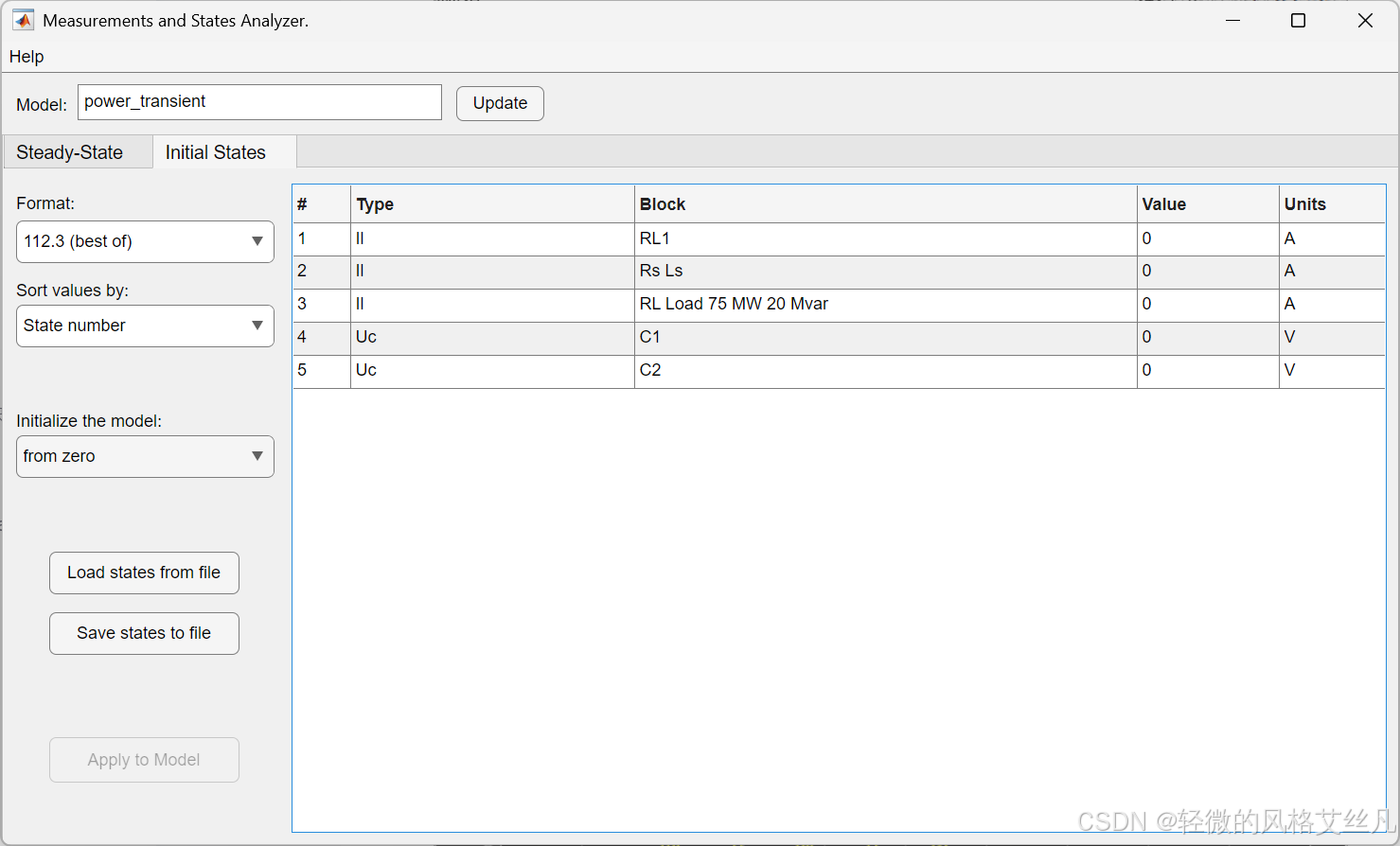
可以设置自定义的初始化内容,注意点击measurements and states analyzer窗口的update和powergui窗口的应用。
离散化
形状大体一致,但在瞬态可以看到离散化的波形在小时间尺度上的阶梯形状。
向量仿真phasor simulation
个人体会不深,引用官方说明:"尤其适用于研究发电机、电动机涉及低频振荡模式的机电暂态过程。"
总结
通过这两个例子,可以初步体会到线性电力系统的模型搭建和学习powergui的阻抗计算,稳态和初态设置,离散仿真,向量仿真等一些用法。