算法：线性回归

模型

模型的概念：经验

天气预报，根据过去数十年天气的特征，对应的天气，建立出模型。然后把新的特征（乌云，风，降温，7月）放模型当中，来预测未来的天气（60%的概率两个小时内有雨）。

公式：

这里的是特征

线性回归

线性回归是一种用于建立因变量（目标变量）与一个或多个自变量（特征变量）之间线性关系的统计模型。它的核心思想是：用一条直线（或一个超平面）来拟合数据点，使得预测值与真实值之间的误差最小。

简单线性回归：只有一个自变量

其中是因变量，是自变量，是截距，是斜率，是误差项。

多元线性回归：有多个自变量

python 复制代码

# 导⼊所需的库
import numpy as np
import matplotlib.pyplot as plt
from sklearn.linear_model import LinearRegression
# ⽣成⼀些示例数据
np.random.seed(0)
X = 2 * np.random.rand(100, 1)
y = 4 + 3 * X + np.random.randn(100, 1)
# 创建线性回归模型
model = LinearRegression()
# 训练模型
model.fit(X, y)
# 获取模型参数
slope = model.coef_[0]
intercept = model.intercept_
# 打印模型参数
print("斜率 (Slope):", slope[0])
print("截距 (Intercept):", intercept[0])
# 绘制数据点和拟合直线
plt.scatter(X, y, color='blue')
plt.plot(X, model.predict(X), color='red', linewidth=3
)
plt.xlabel('X')
plt.ylabel('y')
plt.title('Simple Linear Regression')
plt.show()

模型评估

这是机器学习工作流中至关重要的一环，决定了模型的好坏、是否需要改进以及如何改进

均方误差（MSE）

它衡量的是预测值与真实值之间差异的平方的平均值

是真实值，是预测值，残差（单个样本的误差），是样本数量。每个样本误差的平方求和最后除以样本数量。

均方根误差 (RMSE)

平均平方误差的平方根，即在MSE的基础上，取平方根。

平均绝对误差 (MAE)

平均绝对值误差，为所有样本数据误差的绝对值和

R² (决定系数)

用来表示模型拟合性的分值，值越高表示模型拟合性越好，在训练集中，R^2的取值范围为[0,1]。在测试集（未知数据)中，R^2的取值范围为[-∞,1]。

步骤

1.获取数据集

2.指定特征列和目标列

3.划分数据集：训练集和测试集

4.模型的建立

5.模型的评估

导包

python 复制代码

import matplotlib.pyplot as plt
import numpy as np
from sklearn.linear_model import LinearRegression #线性回归的包
from sklearn.model_selection import train_test_split # 划分数据集的包
from sklearn.datasets import load_iris #鸢尾花的包

如果没有需要安装一下这些包

打印出来看看

python 复制代码

iris=load_iris()
print(iris)

指定特征列和目标列

python 复制代码

X=iris.data[:,2].reshape(-1, 1) #升维处理
y=iris.data[:,3]
print(X)

线性回归+划分数据集

python 复制代码

line=LinearRegression()
X_train,X_test,y_train,y_test=train_test_split(X,y,test_size=0.2,random_state=0)

拟合

python 复制代码

import random

random.seed(4)
nums = [random.randint(1, 100) for i in range(10)]
print(nums)
# todo:拟合
line.fit(X_train, y_train)
print("权重：", line.coef_)
print('截距：', line.intercept_)

预测

python 复制代码

# todo:预测
Y = line.predict(X_test)
print("预测值：", Y)
print('真实值：', y_test)

可视化

python 复制代码

# todo:可视化
plt.figure(figsize=(15, 6))
plt.rcParams['font.family'] = 'SimHei'
plt.plot(y_test, label='真实值', color='red', marker='o')
plt.plot(Y, label='预测值', color='yellow', marker='D')
plt.xlabel('预测集序号')
plt.ylabel('数据值')
plt.legend()
plt.show()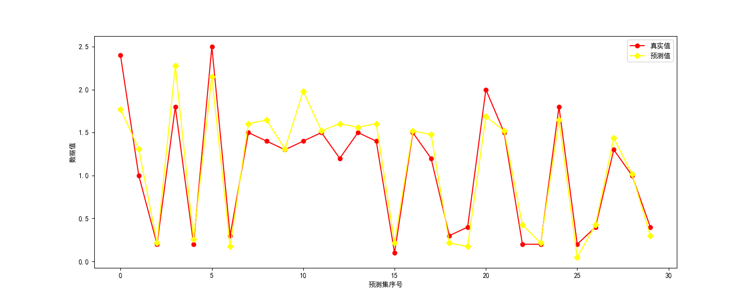

模型评估

python 复制代码

# todo:模型评估
from sklearn.metrics import mean_squared_error, mean_absolute_error, r2_score

print("均方误差：", mean_squared_error(y_test, Y))
print("平均绝对误差：", mean_absolute_error(y_test, Y))
print("训练集:", r2_score(y_train, line.predict(X_train)))
print("测试集：", r2_score(y_test, Y))
print(line.score(X_train, y_train))
print(line.score(X_test, y_test))

多元线性回归

python 复制代码

# todo:多元线性回归
import pandas as pd

df = pd.read_csv('boston_housing_data.csv')  # 波斯顿房价数据集
print(df)

python 复制代码

X = df.drop(columns='MEDV') # todo:方法二:X=data.iloc[:,:-1]  :表示选取所有的行 -1表示选取除了最后一列之外的所有列
y = df['MEDV']
print(X)
print(y)

空值后面报错之后在处理

python 复制代码

print(df.isnull().sum())
print(df['MEDV'].fillna(0, inplace=True))
print(df.isnull().sum())

最后预测

python 复制代码

# todo:多元线性回归
line1 = LinearRegression()
# todo:3.划分数据集：训练集和测试集
X_train, X_test, y_train, y_test = train_test_split(X, y, test_size=0.2, random_state=0)
# todo:拟合
line1.fit(X_train, y_train)
print("权重：", line1.coef_)
print('截距：', line1.intercept_)
# todo:预测
Y = line1.predict(X_test)
print("预测值：", Y)
print('真实值：', y_test)

完整代码

python 复制代码

import matplotlib.pyplot as plt
import numpy as np
import random
from sklearn.linear_model import LinearRegression  # 线性回归的包
from sklearn.model_selection import train_test_split  # 划分数据集的包
from sklearn.datasets import load_iris  # 鸢尾花的包
import pandas as pd

iris = load_iris()
# print(iris)
X = iris.data[:, 2].reshape(-1, 1)  # 升维处理
y = iris.data[:, 3]
# print(X)
# todo:线性回归
line = LinearRegression()
# todo:3.划分数据集：训练集和测试集
X_train, X_test, y_train, y_test = train_test_split(X, y, test_size=0.2, random_state=0)

random.seed(4)
nums = [random.randint(1, 100) for i in range(10)]
print(nums)
# todo:拟合
line.fit(X_train, y_train)
print("权重：", line.coef_)
print('截距：', line.intercept_)

# todo:预测
Y = line.predict(X_test)
print("预测值：", Y)
print('真实值：', y_test)

# todo:可视化
plt.figure(figsize=(15, 6))
plt.rcParams['font.family'] = 'SimHei'
plt.plot(y_test, label='真实值', color='red', marker='o')
plt.plot(Y, label='预测值', color='yellow', marker='D')
plt.xlabel('预测集序号')
plt.ylabel('数据值')
plt.legend()
plt.show()

# todo:模型评估
from sklearn.metrics import mean_squared_error, mean_absolute_error, r2_score

print("均方误差：", mean_squared_error(y_test, Y))
print("平均绝对误差：", mean_absolute_error(y_test, Y))
print("训练集:", r2_score(y_train, line.predict(X_train)))
print("测试集：", r2_score(y_test, Y))
print(line.score(X_train, y_train))
print(line.score(X_test, y_test))

# todo:多元线性回归
df = pd.read_csv('boston_housing_data.csv')  # 波斯顿房价数据集
print(df)


X = df.drop(columns='MEDV')  # todo:方法二:X=data.iloc[:,:-1]  :表示选取所有的行 -1表示选取除了最后一列之外的所有列
y = df['MEDV']
print(X)
print(y)

# todo:空值后面报错之后在处理
print(df.isnull().sum())
print(df['MEDV'].fillna(0, inplace=True))
print(df.isnull().sum())

# todo:多元线性回归
line1 = LinearRegression()
# todo:3.划分数据集：训练集和测试集
X_train, X_test, y_train, y_test = train_test_split(X, y, test_size=0.2, random_state=0)
# todo:拟合
line1.fit(X_train, y_train)
print("权重：", line1.coef_)
print('截距：', line1.intercept_)
# todo:预测
Y = line1.predict(X_test)
print("预测值：", Y)
print('真实值：', y_test)