【深度学习】自动微分模块

深度学习

自动微分模块
- 基本概念
- 梯度基本计算
- 梯度下降法求最优解
- [detach() 函数](#detach() 函数)
- 自动微分应用
- 案例：模拟线性回归

自动微分模块

基本概念

训练神经网络时，最常用的算法就是反向传播。在该算法中，参数（模型权重）会根据损失函数关于对应参数的梯度进行调整。为了计算这些梯度，PyTorch 内置了名为 torch.autograd 的微分模块（通过 backward 方法、grad 属性来实现计算和访问）。它支持任意计算图的自动梯度计算：

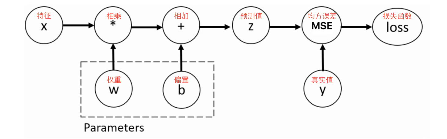
自动微分就是对损失函数求导，结合反向传播，更新权重参数 W、b

梯度下降（Gradient Descent）中对于任意参数 θ \theta θ（权重 W W W 或偏置 b b b），更新公式为：

θ new = θ old − η ⋅ ∇ θ L ( θ old ) \theta_{\text{new}} = \theta_{\text{old}} - \eta \cdot \nabla_{\theta} \mathcal{L}(\theta_{\text{old}}) θnew=θold−η⋅∇θL(θold)

其中：

θ new \theta_{\text{new}} θnew：更新后的参数
θ old \theta_{\text{old}} θold：更新前的参数
η \eta η（学习率）：步长系数（通常取 1 0 − 3 ∼ 1 0 − 5 10^{−3}∼10^{−5} 10−3∼10−5，需通过验证集调优）
∇ θ L \nabla_{\theta} \mathcal{L} ∇θL：损失函数关于 θ \theta θ 的梯度（偏导数）

反向传播就是通过对损失函数求导更新权重，而从特征到预测值的过程则是正向传播

梯度基本计算

PyTorch 不支持向量张量对向量张量的求导，只支持标量张量对向量张量的求导（ x x x 如果是张量， y y y 必须是标亮（一个值）才可以进行求导）

计算梯度：y.backward()， y y y 是一个标量

获取 x x x 点的梯度值：x.grad，会累加上一次的梯度

python 复制代码

import torch

# 1. 定义变量，记录初始的的权重w(旧)
# 参数1: 初始值，参数2: 是否需要自动微分(求导)，参数3: 数据类型
w = torch.tensor(10, requires_grad=True, dtype=torch.float)

# 2. 定义loss变量表示损失函数（模拟）
loss = 2 * w ** 2   # loss = 2w^2 -> 求导：4w

# 3. 打印梯度函数类型（了解）
print(f"梯度函数类型：{type(loss.grad_fn)}")
print(f"loss: {loss.sum()}")

# 4. 对loss进行求导，计算完后会记录到w.grad中
loss.sum().backward()   # 保证loss是标量
# loss.backward()
# 也可以使用该方法求导，因为w本身就是标量，所以效果与backward()相同
print(f"w.grad: {w.grad}")

# 5. 代入权重更新公式
w.data = w.data - 0.01 * w.grad

# 6. 打印更新后的权重w(新)
print(f"更新后的w: {w}")

输出结果如下：

mathematica 复制代码

梯度函数类型：<class 'MulBackward0'>
loss: 200.0
w.grad: 40.0
更新后的w: 9.600000381469727

梯度下降法求最优解

梯度下降法公式： W n e w = W o l d − η ⋅ ∇ W L ( W o l d ) W_{new} = W_{old} - \eta \cdot \nabla_{W} \mathcal{L}(W_{old}) Wnew=Wold−η⋅∇WL(Wold)

清空上一次的梯度值：w.grad.zero()（如果不清空的话每次的梯度都会累加）

python 复制代码

import torch

# 1. 定义点 w=10 requires_grad=True dtype=torch.float
w = torch.tensor(10, requires_grad=True, dtype=torch.float)

# 2. 定义函数 loss = w**2 + 20
loss = w**2 + 20

# 3. 利用梯度下降法，循环迭代10求最优解
print(f"开始 权重初始值：{w}，(0.01 * w.grad)：无，loss：{loss}")
# 循环迭代100求最优解
for i in range(10):
    # 3.1 正向计算（前向传播）
    loss = w**2 + 20

    # 3.2梯度清零
    if w.grad is not None:
        w.grad.zero_()

    # 3.3 反向传播
    loss.backward()

    # 3.4 梯度更新
    print(f"第{i}次迭代 梯度值：{w.grad}")
    w.data = w.data - 0.01 * w.grad

    # 3.5 打印本次梯度更新后的权重参数结果
    print(f"第{i}次迭代 权重值：{w:.5f}，(0.01 * w.grad)：{0.01 * w.grad:.5f}，loss：{loss:.5f}")

# 4. 打印最终结果
print(f"最终 权重值：{w:.5f}，梯度：{w.grad:.5f}，loss：{loss:.5f}")

输出结果如下：

mathematica 复制代码

开始 权重初始值：10.0，(0.01 * w.grad)：无，loss：120.0
第0次迭代 梯度值：20.0
第0次迭代 权重值：9.80000，(0.01 * w.grad)：0.20000，loss：120.00000
第1次迭代 梯度值：19.600000381469727
第1次迭代 权重值：9.60400，(0.01 * w.grad)：0.19600，loss：116.04000
第2次迭代 梯度值：19.20800018310547
第2次迭代 权重值：9.41192，(0.01 * w.grad)：0.19208，loss：112.23682
第3次迭代 梯度值：18.823841094970703
第3次迭代 权重值：9.22368，(0.01 * w.grad)：0.18824，loss：108.58425
第4次迭代 梯度值：18.447364807128906
第4次迭代 权重值：9.03921，(0.01 * w.grad)：0.18447，loss：105.07632
第5次迭代 梯度值：18.07841682434082
第5次迭代 权重值：8.85842，(0.01 * w.grad)：0.18078，loss：101.70729
第6次迭代 梯度值：17.716848373413086
第6次迭代 权重值：8.68126，(0.01 * w.grad)：0.17717，loss：98.47168
第7次迭代 梯度值：17.362510681152344
第7次迭代 权重值：8.50763，(0.01 * w.grad)：0.17363，loss：95.36420
第8次迭代 梯度值：17.015260696411133
第8次迭代 权重值：8.33748，(0.01 * w.grad)：0.17015，loss：92.37978
第9次迭代 梯度值：16.674955368041992
第9次迭代 权重值：8.17073，(0.01 * w.grad)：0.16675，loss：89.51353
最终 权重值：8.17073，梯度：16.67496，loss：89.51353

detach() 函数

自动微分存在的问题：一个张量一旦设置了自动微分，就无法直接转换成 Numpy 的 ndarray 对象

这种情况就需要用 detach() 函数来解决

python 复制代码

import torch
import numpy as np

# 1，定义张量
t1 = torch.tensor([10, 20], dtype =torch.float)
t2 = torch.tensor([20, 30], requires_grad=True, dtype =torch.float)
print(f"t1:{t1},type:{type(t1)}")
print(f"t2:{t2},type:{type(t2)}")

# 2.尝试把张量 t1 转换为 numpy ndarray 对象
n1 = t1.numpy()
print(f"n1: {n1},type:{type(n1)}")

# 3. 尝试把张量 t2 转换为 numpy ndarray 对象
# n2 = t2.numpy()
# print(f"n2: {n2},type:{type(n2)}")
# 报错：Traceback (most recent call last):
#   File "/Users/PycharmProjects/DL_learn/day03/03_自动微分模块_detach函数.py", line 20, in <module>
#     n2 = t2.numpy()
#          ^^^^^^^^^^
# RuntimeError: Can't call numpy() on Tensor that requires grad. Use tensor.detach().numpy() instead.

# 4. 尝试把张量 t2 转换为 numpy ndarray 对象，使用 detach() 函数
t3 = t2.detach()
print(f"t3: {t3},type:{type(t3)}")
# 测试：t3 是否与 t2 共享内存
t3[0] = 100
print(f"t3: {t3}")
print(f"t2: {t2}")
# 查看 t2 和 t3 哪个可以自动微分
print(f"t2.requires_grad: {t2.requires_grad}")
print(f"t3.requires_grad: {t3.requires_grad}")

n2 = t3.numpy()
print(f"n2: {n2},type:{type(n2)}")

输出结果如下：

mathematica 复制代码

t1:tensor([10., 20.]),type:<class 'torch.Tensor'>
t2:tensor([20., 30.], requires_grad=True),type:<class 'torch.Tensor'>
n1: [10. 20.],type:<class 'numpy.ndarray'>
t3: tensor([20., 30.]),type:<class 'torch.Tensor'>
t3: tensor([100.,  30.])
t2: tensor([100.,  30.], requires_grad=True)
t2.requires_grad: True
t3.requires_grad: False
n2: [100.  30.],type:<class 'numpy.ndarray'>

自动微分应用

python 复制代码

import torch

# 1. 定义x，表示：特征（输入数据），假设：2行5列的全1矩阵
x = torch.ones(2, 5)
print(f"x: {x}")

# 2. 定义y，表示：标签（真实值），假设：2行3列的全0矩阵
y = torch.zeros(2, 3)
print(f"y: {y}")

# 3. 初始化（可自动微分的）权重和偏置
w = torch.randn(5, 3, requires_grad=True)
print(f"w: {w}")
b = torch.randn(3, requires_grad=True)
print(f"b: {b}")

# 新建一个 MSELoss 对象
criterion = torch.nn.MSELoss()

# 设置学习率
learning_rate = 0.01

for i in range(10):
    # 4. 前向传播计算出预测值（每次迭代都需要重新计算）
    z = torch.matmul(x, w) + b
    
    # 5. 定义损失函数
    loss = criterion(z, y)

    # 6. 梯度清零
    if w.grad is not None:
        w.grad.data.zero_()
    if b.grad is not None:
        b.grad.data.zero_()

    # 7. 计算损失函数关于权重和偏置的梯度
    loss.backward()
    print(f"第{i}次迭代：")
    print(f"w.grad: {w.grad}")
    print(f"b.grad: {b.grad}")

    # 8. 基于梯度，更新权重和偏置
    with torch.no_grad():
        w.data -= learning_rate * w.grad
        b.data -= learning_rate * b.grad

    # 打印本次梯度更新后的权重参数结果
    print(f"权重值w：{w}，偏置值b：{b}")
    print(f"损失函数值loss：{loss}")

输出结果如下：

mathematica 复制代码

x: tensor([[1., 1., 1., 1., 1.],
        [1., 1., 1., 1., 1.]])
y: tensor([[0., 0., 0.],
        [0., 0., 0.]])
w: tensor([[ 0.1683, -1.3922,  0.0113],
        [-0.3075, -0.5632,  0.1783],
        [ 0.6182, -0.4339, -1.5849],
        [-1.3927, -0.1006,  1.0168],
        [-0.4363, -0.7434, -0.3629]], requires_grad=True)
b: tensor([-1.4458, -0.6056, -1.8829], requires_grad=True)
第0次迭代：
w.grad: tensor([[-1.8639, -2.5593, -1.7495],
        [-1.8639, -2.5593, -1.7495],
        [-1.8639, -2.5593, -1.7495],
        [-1.8639, -2.5593, -1.7495],
        [-1.8639, -2.5593, -1.7495]])
b.grad: tensor([-1.8639, -2.5593, -1.7495])
权重值w：tensor([[ 0.1870, -1.3666,  0.0288],
        [-0.2889, -0.5376,  0.1958],
        [ 0.6368, -0.4083, -1.5674],
        [-1.3741, -0.0750,  1.0343],
        [-0.4177, -0.7178, -0.3454]], requires_grad=True)，偏置值b：tensor([-1.4272, -0.5800, -1.8654], requires_grad=True)
损失函数值loss：9.813471794128418
第1次迭代：
w.grad: tensor([[-1.7893, -2.4569, -1.6795],
        [-1.7893, -2.4569, -1.6795],
        [-1.7893, -2.4569, -1.6795],
        [-1.7893, -2.4569, -1.6795],
        [-1.7893, -2.4569, -1.6795]])
b.grad: tensor([-1.7893, -2.4569, -1.6795])
权重值w：tensor([[ 0.2049, -1.3421,  0.0456],
        [-0.2710, -0.5130,  0.2126],
        [ 0.6547, -0.3837, -1.5506],
        [-1.3562, -0.0504,  1.0511],
        [-0.3998, -0.6932, -0.3286]], requires_grad=True)，偏置值b：tensor([-1.4093, -0.5555, -1.8486], requires_grad=True)
损失函数值loss：9.044095993041992
第2次迭代：
w.grad: tensor([[-1.7177, -2.3586, -1.6123],
        [-1.7177, -2.3586, -1.6123],
        [-1.7177, -2.3586, -1.6123],
        [-1.7177, -2.3586, -1.6123],
        [-1.7177, -2.3586, -1.6123]])
b.grad: tensor([-1.7177, -2.3586, -1.6123])
权重值w：tensor([[ 0.2221, -1.3185,  0.0617],
        [-0.2538, -0.4895,  0.2287],
        [ 0.6719, -0.3601, -1.5345],
        [-1.3390, -0.0268,  1.0673],
        [-0.3826, -0.6696, -0.3125]], requires_grad=True)，偏置值b：tensor([-1.3921, -0.5319, -1.8325], requires_grad=True)
损失函数值loss：8.335038185119629
第3次迭代：
w.grad: tensor([[-1.6490, -2.2643, -1.5478],
        [-1.6490, -2.2643, -1.5478],
        [-1.6490, -2.2643, -1.5478],
        [-1.6490, -2.2643, -1.5478],
        [-1.6490, -2.2643, -1.5478]])
b.grad: tensor([-1.6490, -2.2643, -1.5478])
权重值w：tensor([[ 0.2385, -1.2958,  0.0772],
        [-0.2373, -0.4668,  0.2442],
        [ 0.6884, -0.3375, -1.5190],
        [-1.3225, -0.0042,  1.0827],
        [-0.3661, -0.6470, -0.2970]], requires_grad=True)，偏置值b：tensor([-1.3756, -0.5092, -1.8170], requires_grad=True)
损失函数值loss：7.6815714836120605
第4次迭代：
w.grad: tensor([[-1.5831, -2.1737, -1.4859],
        [-1.5831, -2.1737, -1.4859],
        [-1.5831, -2.1737, -1.4859],
        [-1.5831, -2.1737, -1.4859],
        [-1.5831, -2.1737, -1.4859]])
b.grad: tensor([-1.5831, -2.1737, -1.4859])
权重值w：tensor([[ 0.2544, -1.2741,  0.0920],
        [-0.2215, -0.4451,  0.2591],
        [ 0.7042, -0.3157, -1.5041],
        [-1.3067,  0.0175,  1.0976],
        [-0.3503, -0.6253, -0.2822]], requires_grad=True)，偏置值b：tensor([-1.3598, -0.4875, -1.8022], requires_grad=True)
损失函数值loss：7.0793375968933105
第5次迭代：
w.grad: tensor([[-1.5198, -2.0868, -1.4265],
        [-1.5198, -2.0868, -1.4265],
        [-1.5198, -2.0868, -1.4265],
        [-1.5198, -2.0868, -1.4265],
        [-1.5198, -2.0868, -1.4265]])
b.grad: tensor([-1.5198, -2.0868, -1.4265])
权重值w：tensor([[ 0.2696, -1.2532,  0.1063],
        [-0.2063, -0.4242,  0.2733],
        [ 0.7194, -0.2949, -1.4899],
        [-1.2915,  0.0384,  1.1119],
        [-0.3351, -0.6044, -0.2679]], requires_grad=True)，偏置值b：tensor([-1.3446, -0.4666, -1.7879], requires_grad=True)
损失函数值loss：6.524317264556885
第6次迭代：
w.grad: tensor([[-1.4590, -2.0033, -1.3694],
        [-1.4590, -2.0033, -1.3694],
        [-1.4590, -2.0033, -1.3694],
        [-1.4590, -2.0033, -1.3694],
        [-1.4590, -2.0033, -1.3694]])
b.grad: tensor([-1.4590, -2.0033, -1.3694])
权重值w：tensor([[ 0.2842, -1.2332,  0.1200],
        [-0.1917, -0.4042,  0.2870],
        [ 0.7340, -0.2748, -1.4762],
        [-1.2769,  0.0584,  1.1255],
        [-0.3205, -0.5844, -0.2542]], requires_grad=True)，偏置值b：tensor([-1.3300, -0.4466, -1.7742], requires_grad=True)
损失函数值loss：6.012809753417969
第7次迭代：
w.grad: tensor([[-1.4006, -1.9232, -1.3147],
        [-1.4006, -1.9232, -1.3147],
        [-1.4006, -1.9232, -1.3147],
        [-1.4006, -1.9232, -1.3147],
        [-1.4006, -1.9232, -1.3147]])
b.grad: tensor([-1.4006, -1.9232, -1.3147])
权重值w：tensor([[ 0.2982, -1.2140,  0.1331],
        [-0.1777, -0.3849,  0.3002],
        [ 0.7480, -0.2556, -1.4630],
        [-1.2629,  0.0777,  1.1387],
        [-0.3065, -0.5651, -0.2411]], requires_grad=True)，偏置值b：tensor([-1.3160, -0.4274, -1.7610], requires_grad=True)
损失函数值loss：5.541406154632568
第8次迭代：
w.grad: tensor([[-1.3446, -1.8462, -1.2621],
        [-1.3446, -1.8462, -1.2621],
        [-1.3446, -1.8462, -1.2621],
        [-1.3446, -1.8462, -1.2621],
        [-1.3446, -1.8462, -1.2621]])
b.grad: tensor([-1.3446, -1.8462, -1.2621])
权重值w：tensor([[ 0.3116, -1.1955,  0.1458],
        [-0.1642, -0.3665,  0.3128],
        [ 0.7615, -0.2371, -1.4504],
        [-1.2494,  0.0961,  1.1513],
        [-0.2930, -0.5467, -0.2284]], requires_grad=True)，偏置值b：tensor([-1.3026, -0.4089, -1.7484], requires_grad=True)
损失函数值loss：5.106959819793701
第9次迭代：
w.grad: tensor([[-1.2908, -1.7724, -1.2116],
        [-1.2908, -1.7724, -1.2116],
        [-1.2908, -1.7724, -1.2116],
        [-1.2908, -1.7724, -1.2116],
        [-1.2908, -1.7724, -1.2116]])
b.grad: tensor([-1.2908, -1.7724, -1.2116])
权重值w：tensor([[ 0.3245, -1.1778,  0.1579],
        [-0.1513, -0.3488,  0.3249],
        [ 0.7744, -0.2194, -1.4383],
        [-1.2365,  0.1139,  1.1634],
        [-0.2801, -0.5289, -0.2163]], requires_grad=True)，偏置值b：tensor([-1.2897, -0.3912, -1.7363], requires_grad=True)
损失函数值loss：4.706573963165283

案例：模拟线性回归

在 Pytorch 中进行模型构建的整个流程一般分为四个步骤：

准备训练集数据
构建要使用的模型
设置损失函数和优化器
模型训练

使用到的 API：

使用 Pytorch 的 nn.MSELoss() 代替平方损失函数
使用 Pytorch 的 data.DataLoader 代替数据加载器
使用 Pytorch 的 optim.SGD 代替优化器
使用 Pytorch 的 nn.Linear 代替假设函数

python 复制代码

import torch
from torch.utils.data import TensorDataset   # 构造数据集对象
from torch.utils.data import DataLoader      # 构造数据加载器对象
# numpy对象 -> 张量Tensor -> 数据集Dataset -> 数据加载器DataLoader
from torch import nn                         # 神经网络模块
from torch import optim                      # 优化器模块
from sklearn.datasets import make_regression # 生成模拟回归数据集
import matplotlib.pyplot as plt

plt.rcParams['font.sans-serif'] = ['Arial Unicode MS', 'SimHei', 'DejaVu Sans'] # 用来正常显示中文标签
plt.rcParams['axes.unicode_minus'] = False    # 用来正常显示负号

# 定义函数，创建线性回归样本数据
def create_dataset():
    # 创建数据集对象
    x, y, coef = make_regression(n_samples=100, # 样本数量100
                                 n_features=1, # 特征数量1
                                 noise=10, # 噪声，噪声越大，样本数据越散，噪声越小，样本数据越集中
                                 coef=True, # 是否返回系数，默认False，返回为None
                                 bias=14.5, # 偏置项
                                 random_state=3) # 随机种子
    print(f"x_type:{type(x)},y_type:{type(y)},coef_type:{type(coef)}")

    # 将构建数据转换为张量类型
    x = torch.tensor(x, dtype=torch.float)
    y = torch.tensor(y, dtype=torch.float)

    return x, y, coef

# 定义函数，表示模型训练
def train(x, y, coef):
    # 1. 构造数据集对象
    dataset = TensorDataset(x, y)
    # 2. 构造数据加载器对象
    # 参数1: 数据集对象，参数2: 批次大小，默认1，参数3: 是否打乱数据，默认False（训练集打乱，测试集不打乱）
    dataloader = DataLoader(dataset, batch_size=16, shuffle=True)
    # 3. 创建初始的线性回归模型
    # 参数1: 输入特征数量，参数2: 输出特征数量
    model = nn.Linear(1, 1)
    # 4. 创建损失函数对象
    criterion = nn.MSELoss()
    # 5. 创建优化器对象
    # 参数1: 模型参数，参数2: 学习率
    optimizer = optim.SGD(model.parameters(), lr=0.01)
    # 6. 具体的训练过程
    # 6.1 定义变量，分别表示：训练轮数，每轮的（平均）损失值，训练总损失值，训练的样本数
    epochs, loss_list, total_loss, total_samples = 100, [], 0, 0
    # 6.2 开始训练，按轮训练
    for epoch in range(epochs):
        # 6.2.1 每轮是分批次训练的，从数据加载器中获取批次数据
        for train_x, train_y in dataloader: # 7批（16，16，16，16，16，16，4）
            # 6.2.1.1 模型预测
            y_pred = model(train_x)
            # 6.2.1.2 计算（每批的平均）损失值
            loss = criterion(y_pred, train_y.reshape(-1, 1)) # -1 表示自动计算
            # 6.2.1.3 计算总损失和样本（批次）数
            total_loss += loss.item()
            total_samples += 1
            # 6.2.1.4 梯度清零，反向传播，梯度更新
            optimizer.zero_grad()   # 梯度清零
            loss.backward()         # 反向传播，计算梯度
            optimizer.step()        # 梯度更新
        # 6.2.2 把本轮的（平均）损失值，添加到列表中
        loss_list.append(total_loss / total_samples)
        print(f"epoch:{epoch+1},loss:{total_loss / total_samples}")
    # 7. 打印最终的训练结果
    print(f"{epochs}轮的平均损失值为：{loss_list}")
    print(f"模型参数，权重：{model.weight.item()}，偏置：{model.bias.item()}")

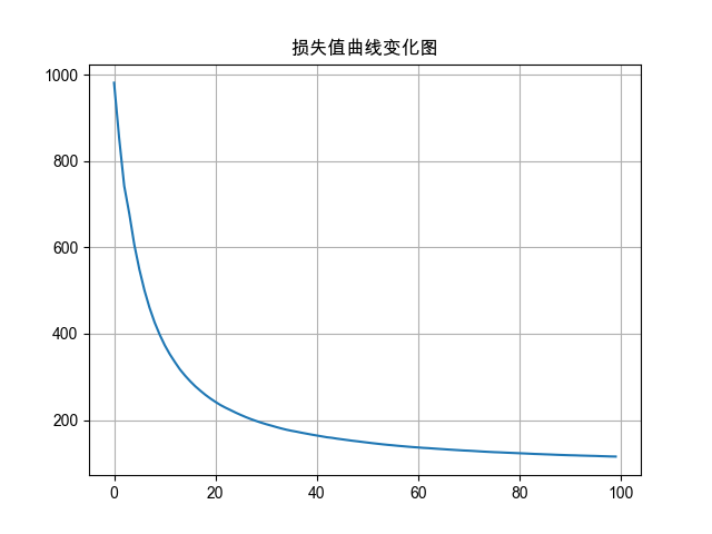
    # 8. 绘制损失曲线
    plt.plot(range(epochs), loss_list)
    plt.title('损失值曲线变化图')
    plt.grid()  # 显示网格线
    plt.show()  # 显示损失曲线

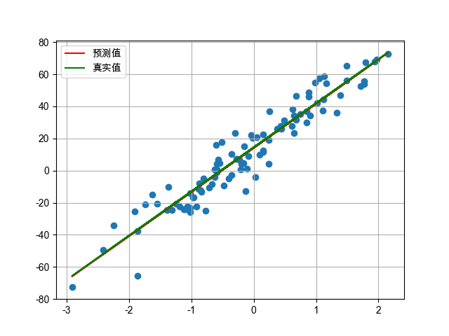
    # 9. 绘制预测值和真实值的关系
    # 绘制样本点分布情况
    plt.scatter(x, y)
    # 绘制训练模型的预测值
    y_pred = torch.tensor(data = [v * model.weight.item() + model.bias.item() for v in x])
    # 计算真实值
    y_true = torch.tensor(data = [v * coef.item() + 14.5 for v in x])
    # 绘制预测值和真实值的折线图
    plt.plot(x, y_pred, color='red', label='预测值')
    plt.plot(x, y_true, color='green', label='真实值')
    plt.legend()  # 显示图例
    plt.grid()  # 显示网格线
    plt.show()

if __name__ == "__main__":

    # 创建数据集
    x, y, coef = create_dataset()
    # print(f"x_shape:{x.shape},y_shape:{y.shape},coef_shape:{coef.shape}")
    # print(f"x:{x},y:{y},coef:{coef}")

    # 模型训练
    train(x, y, coef)

输出结果如下：

mathematica 复制代码

epoch:1,loss:981.5269252232143
epoch:2,loss:853.3959612165179
epoch:3,loss:742.5516124906994
...
epoch:98,loss:116.04389740774305
epoch:99,loss:115.62916484436431
epoch:100,loss:115.40643576894487
100轮的平均损失值为：[981.5269252232143, 853.3959612165179, 742.5516124906994, 678.4569364275251, 605.8102375575475, 548.6587242853074, 500.36826098695093, 460.1560640675681, 426.3043611011808, 398.0191957473755, 373.3733908665645, 352.55637702487763, 334.41243330986947, 317.3166756338003, 303.06303981599353, 290.23163395268574, 278.5381171122319, 268.30006616077725, 258.62909295505153, 249.9824803352356, 242.1277265873085, 234.78329686994675, 228.59299124249762, 222.9695519379207, 217.2016434914725, 211.90159880459964, 206.87735432417935, 202.21674172732295, 198.0625297377262, 194.10351158323743, 190.4825868826308, 187.20595926046371, 183.82109612303896, 180.60866456873276, 177.6812167887785, 175.193129478939, 173.06181149869352, 170.65958882095222, 168.4760366726271, 166.26354225703648, 164.24055067587398, 162.20579415924695, 160.15612860454672, 158.80201498564188, 156.93153119465663, 155.34386212781348, 153.73787305130423, 152.13456554356077, 150.77345948455633, 149.30770564215524, 147.8670169365506, 146.433272254336, 145.1130473273141, 143.80517857919926, 142.58734095437185, 141.55579608070607, 140.3645850351281, 139.37626582178575, 138.30676883762166, 137.38113928295317, 136.51254849579072, 135.57208513004989, 134.959542306913, 134.11099514790945, 133.27229425618935, 132.48517642495952, 131.70074998900327, 130.94415850599273, 130.21998091514067, 129.4918162053945, 128.99063432720345, 128.32033567579967, 127.57748236908138, 126.84413563975036, 126.2349357405163, 125.64247574662804, 125.21943763103025, 124.65178913947864, 124.13279057238891, 123.62976352998189, 123.14717520019154, 122.64006108440174, 122.07807005292987, 121.50720818999673, 121.1260860427087, 120.64489899600463, 120.23127605801537, 119.70435118520415, 119.2549658311504, 118.85111155585638, 118.458202333615, 118.2068915233849, 117.74867322807488, 117.4586065011184, 117.11785009427179, 116.85318271460987, 116.40885656887723, 116.04389740774305, 115.62916484436431, 115.40643576894487]
模型参数，权重：27.481021881103516，偏置：14.157599449157715