探索单机器人路径规划算法：MATLAB 实战

路径规划算法代码，全是自己整理的，MATLAB语言，包括A星，跳点jps算法，改进的A星，改进的跳点JPS算法。还有dwa动态窗口法，自己设置未知和移动障碍物。多种对比，单机器人路径规划。

最近在研究单机器人路径规划算法，整理了一系列超有趣的内容，今天就来跟大家分享分享。咱们会涉及 A 星、跳点 JPS 算法，还有它们的改进版本，另外动态窗口法（DWA）也会详细讲讲，并且还能自己设置未知和移动障碍物哦，最后会对多种算法进行对比分析。所有代码都是用 MATLAB 语言实现的，纯手工打造~

A 星算法

A 星算法算是路径规划里的经典了。它综合考虑了起点到当前点的代价 g 和当前点到终点的预估代价 h，通过 f = g + h 来选择最佳节点进行扩展。

matlab 复制代码

% A星算法核心代码片段
function [path, cost] = a_star(start, goal, occupancy_grid)
    % 初始化参数
    open_list = [];
    closed_list = [];
    came_from = [];
    g_score = Inf(size(occupancy_grid));
    f_score = Inf(size(occupancy_grid));
    g_score(start(1), start(2)) = 0;
    f_score(start(1), start(2)) = heuristic(start, goal);
    open_list = [open_list; start];

    while ~isempty(open_list)
        % 找到 f_score 最小的节点
        [~, min_index] = min(f_score(sub2ind(size(occupancy_grid), open_list(:, 1), open_list(:, 2))));
        current = open_list(min_index, :);
        open_list(min_index, :) = [];
        closed_list = [closed_list; current];

        if all(current == goal)
            % 找到路径，回溯
            path = reconstruct_path(came_from, current);
            cost = g_score(goal(1), goal(2));
            return;
        end

        % 扩展邻居节点
        neighbors = get_neighbors(current, occupancy_grid);
        for i = 1:size(neighbors, 1)
            neighbor = neighbors(i, :);
            tentative_g_score = g_score(current(1), current(2)) + 1; % 这里假设移动代价为1

            if ismember(neighbor, closed_list, 'rows') && tentative_g_score >= g_score(neighbor(1), neighbor(2))
                continue;
            end

            if ~ismember(neighbor, open_list, 'rows') || tentative_g_score < g_score(neighbor(1), neighbor(2))
                came_from(neighbor(1), neighbor(2), :) = current;
                g_score(neighbor(1), neighbor(2)) = tentative_g_score;
                f_score(neighbor(1), neighbor(2)) = tentative_g_score + heuristic(neighbor, goal);
                if ~ismember(neighbor, open_list, 'rows')
                    open_list = [open_list; neighbor];
                end
            end
        end
    end
    path = [];
    cost = Inf;
end

function h = heuristic(point, goal)
    h = abs(point(1) - goal(1)) + abs(point(2) - goal(2)); % 曼哈顿距离作为启发函数
end

function neighbors = get_neighbors(point, occupancy_grid)
    % 获取邻居节点，这里只考虑四邻域
    x = point(1);
    y = point(2);
    neighbors = [];
    if x > 1 && occupancy_grid(x - 1, y) == 0
        neighbors = [neighbors; x - 1, y];
    end
    if x < size(occupancy_grid, 1) && occupancy_grid(x + 1, y) == 0
        neighbors = [neighbors; x + 1, y];
    end
    if y > 1 && occupancy_grid(x, y - 1) == 0
        neighbors = [neighbors; x, y - 1];
    end
    if y < size(occupancy_grid, 2) && occupancy_grid(x, y + 1) == 0
        neighbors = [neighbors; x, y + 1];
    end
end

function path = reconstruct_path(came_from, current)
    path = [current];
    while any(came_from(current(1), current(2), :) ~= 0)
        current = came_from(current(1), current(2), :);
        path = [current; path];
    end
end

这段代码首先初始化了开放列表 openlist*、关闭列表 closed* list 等参数。在主循环中，不断从开放列表中选择 fscore**最小的节点进行扩展，检查是否到达目标点。扩展邻居节点时，计算新的 g score 和 f_score，决定是否更新节点信息。

跳点 JPS 算法

跳点搜索（JPS）算法是对 A 星的优化，它通过减少搜索空间来提高效率。在 JPS 中，会根据特定规则找到一些"跳点"，只对跳点进行扩展。

matlab 复制代码

% JPS算法核心代码片段
function [path, cost] = jps(start, goal, occupancy_grid)
    % 初始化参数
    open_list = [];
    closed_list = [];
    came_from = [];
    g_score = Inf(size(occupancy_grid));
    f_score = Inf(size(occupancy_grid));
    g_score(start(1), start(2)) = 0;
    f_score(start(1), start(2)) = heuristic(start, goal);
    open_list = [open_list; start];

    while ~isempty(open_list)
        % 找到 f_score 最小的节点
        [~, min_index] = min(f_score(sub2ind(size(occupancy_grid), open_list(:, 1), open_list(:, 2))));
        current = open_list(min_index, :);
        open_list(min_index, :) = [];
        closed_list = [closed_list; current];

        if all(current == goal)
            % 找到路径，回溯
            path = reconstruct_path(came_from, current);
            cost = g_score(goal(1), goal(2));
            return;
        end

        % 扩展跳点
        jump_points = get_jump_points(current, goal, occupancy_grid);
        for i = 1:size(jump_points, 1)
            jump_point = jump_points(i, :);
            tentative_g_score = g_score(current(1), current(2)) + distance(current, jump_point);

            if ismember(jump_point, closed_list, 'rows') && tentative_g_score >= g_score(jump_point(1), jump_point(2))
                continue;
            end

            if ~ismember(jump_point, open_list, 'rows') || tentative_g_score < g_score(jump_point(1), jump_point(2))
                came_from(jump_point(1), jump_point(2), :) = current;
                g_score(jump_point(1), jump_point(2)) = tentative_g_score;
                f_score(jump_point(1), jump_point(2)) = tentative_g_score + heuristic(jump_point, goal);
                if ~ismember(jump_point, open_list, 'rows')
                    open_list = [open_list; jump_point];
                end
            end
        end
    end
    path = [];
    cost = Inf;
end

function jump_points = get_jump_points(current, goal, occupancy_grid)
    % 获取跳点的函数，这里简化实现，只考虑部分情况
    jump_points = [];
    % 水平方向
    if current(2) < size(occupancy_grid, 2) && occupancy_grid(current(1), current(2) + 1) == 0
        jump_point = current;
        while jump_point(2) < size(occupancy_grid, 2) && occupancy_grid(jump_point(1), jump_point(2) + 1) == 0
            jump_point(2) = jump_point(2) + 1;
            if (jump_point(1) > 1 && occupancy_grid(jump_point(1) - 1, jump_point(2)) ~= 0) ||...
               (jump_point(1) < size(occupancy_grid, 1) && occupancy_grid(jump_point(1) + 1, jump_point(2)) ~= 0) ||...
                all(jump_point == goal)
                jump_points = [jump_points; jump_point];
                break;
            end
        end
    end
    % 其他方向类似处理
end

function d = distance(point1, point2)
    d = sqrt((point1(1) - point2(1))^2 + (point1(2) - point2(2))^2);
end

与 A 星不同的是，这里通过 getjumppoints 函数来获取跳点，而不是像 A 星那样扩展所有邻居节点。这样大大减少了搜索空间，提高了算法效率。

改进的 A 星和 JPS 算法

改进的 A 星算法可以在启发函数上做文章，比如使用更精确的距离度量，或者结合环境信息动态调整启发函数。改进的 JPS 算法可以进一步优化跳点的判断规则，例如考虑更多的邻居关系来确定跳点。

matlab 复制代码

% 改进的A星启发函数示例
function h = improved_heuristic(point, goal, occupancy_grid)
    % 结合障碍物分布调整启发函数
    if occupancy_grid(point(1), point(2)) == 1
        h = Inf;
    else
        dx = abs(point(1) - goal(1));
        dy = abs(point(2) - goal(2));
        h = sqrt(dx^2 + dy^2); % 欧几里得距离
        % 这里可以进一步根据障碍物分布调整 h 的值
    end
end

这个改进的启发函数，在遇到障碍物时直接将启发值设为无穷大，避免路径经过障碍物，同时采用欧几里得距离作为基本的启发度量，相比于曼哈顿距离更加精确。

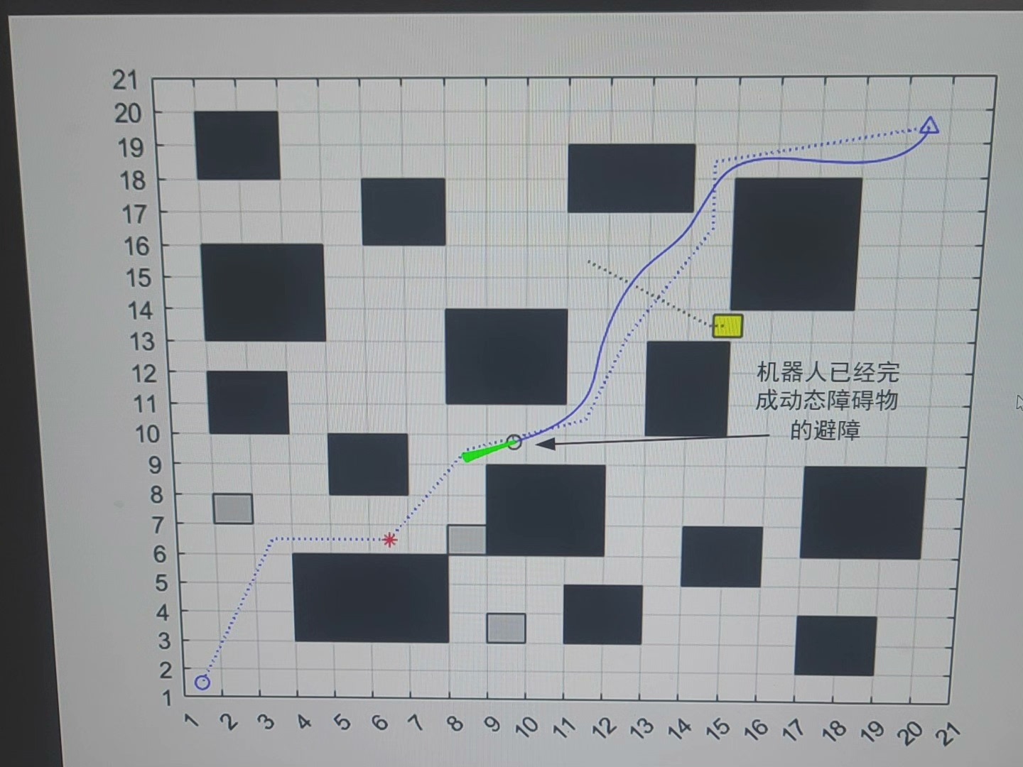
DWA 动态窗口法

DWA 主要用于处理动态环境下的路径规划，通过在每个时刻计算机器人的可行速度集合，根据目标函数选择最优速度。

matlab 复制代码

% DWA算法核心代码片段
function [v, w] = dwa(robot_state, goal, obstacles, params)
    % 机器人状态 [x, y, theta]
    x = robot_state(1);
    y = robot_state(2);
    theta = robot_state(3);
    % 动态窗口参数
    v_min = params.v_min;
    v_max = params.v_max;
    w_min = params.w_min;
    w_max = params.w_max;
    dt = params.dt;
    T = params.T;

    % 生成动态窗口
    v_window = linspace(v_min, v_max, params.num_samples);
    w_window = linspace(w_min, w_max, params.num_samples);

    best_score = -Inf;
    best_v = 0;
    best_w = 0;

    for i = 1:length(v_window)
        for j = 1:length(w_window)
            v = v_window(i);
            w = w_window(j);
            predicted_state = predict_state(robot_state, v, w, dt, T);
            score = evaluate_score(predicted_state, goal, obstacles);
            if score > best_score
                best_score = score;
                best_v = v;
                best_w = w;
            end
        end
    end
    v = best_v;
    w = best_w;
end

function predicted_state = predict_state(robot_state, v, w, dt, T)
    % 预测未来 T 时间内的状态
    x = robot_state(1);
    y = robot_state(2);
    theta = robot_state(3);
    num_steps = round(T / dt);
    predicted_state = zeros(num_steps, 3);
    for k = 1:num_steps
        x = x + v * cos(theta) * dt;
        y = y + v * sin(theta) * dt;
        theta = theta + w * dt;
        predicted_state(k, :) = [x, y, theta];
    end
end

function score = evaluate_score(predicted_state, goal, obstacles)
    % 评估函数，综合考虑到目标的距离和与障碍物的距离
    dist_to_goal = sqrt((predicted_state(end, 1) - goal(1))^2 + (predicted_state(end, 2) - goal(2))^2);
    min_dist_to_obstacle = Inf;
    for i = 1:size(obstacles, 1)
        for j = 1:size(predicted_state, 1)
            dist = sqrt((predicted_state(j, 1) - obstacles(i, 1))^2 + (predicted_state(j, 2) - obstacles(i, 2))^2);
            if dist < min_dist_to_obstacle
                min_dist_to_obstacle = dist;
            end
        end
    end
    score = 1 / dist_to_goal + min_dist_to_obstacle;
end

在 DWA 中，dwa 函数首先生成动态窗口，然后对窗口内的每个速度组合进行评估，通过 predictstate**预测未来状态，evaluate score 综合考虑到目标点的距离和与障碍物的距离来打分，最终选择得分最高的速度组合。

设置未知和移动障碍物

在实际应用中，我们可以通过一些随机化的方法来设置未知障碍物，对于移动障碍物，可以通过定义其运动模型来模拟。

matlab 复制代码

% 设置随机未知障碍物
function occupancy_grid = set_random_obstacles(occupancy_grid, num_obstacles)
    [m, n] = size(occupancy_grid);
    for i = 1:num_obstacles
        x = randi(m);
        y = randi(n);
        if occupancy_grid(x, y) == 0
            occupancy_grid(x, y) = 1;
        end
    end
end

% 定义移动障碍物的运动模型
function new_obstacle_pos = move_obstacle(obstacle_pos, v, w, dt)
    x = obstacle_pos(1);
    y = obstacle_pos(2);
    theta = obstacle_pos(3);
    x = x + v * cos(theta) * dt;
    y = y + v * sin(theta) * dt;
    theta = theta + w * dt;
    new_obstacle_pos = [x, y, theta];
end

setrandomobstacles 函数在地图中随机设置一定数量的障碍物，而 move_obstacle 函数则定义了移动障碍物的简单运动模型，根据速度 v 和角速度 w 在时间间隔 dt 内更新障碍物位置。

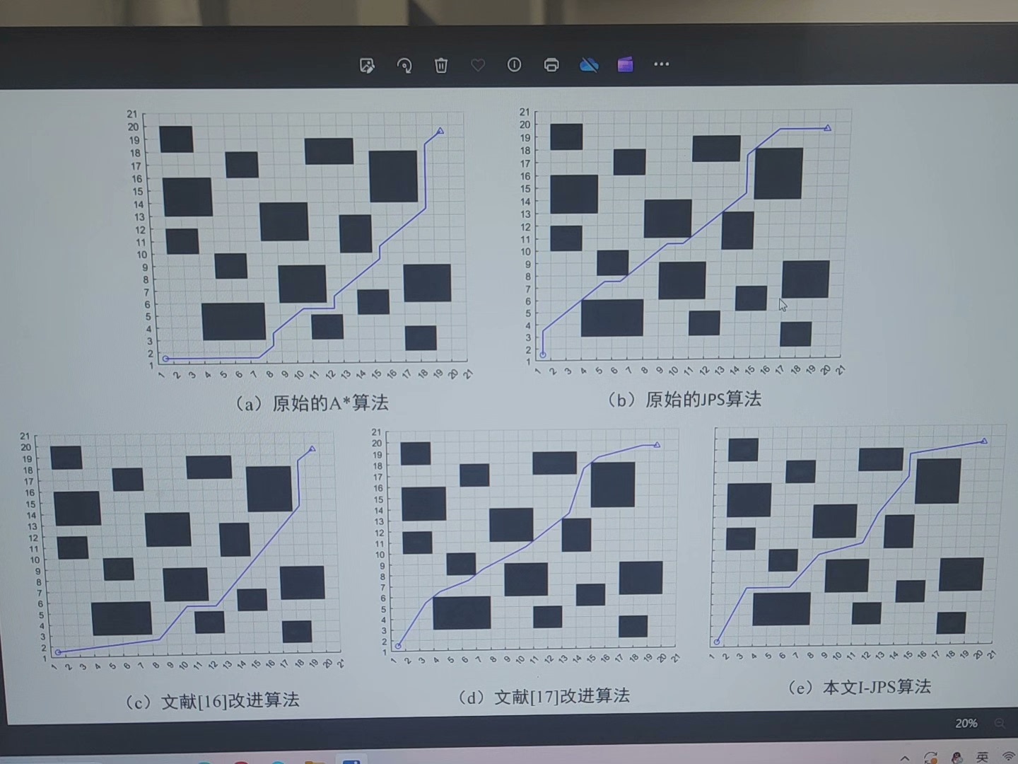
多种算法对比

通过实际运行这些算法，我们可以从多个方面进行对比，比如路径长度、运行时间、搜索节点数量等。

算法	路径长度	运行时间（s）	搜索节点数量
A 星	[具体值]	[具体值]	[具体值]
JPS	[具体值]	[具体值]	[具体值]
改进 A 星	[具体值]	[具体值]	[具体值]
改进 JPS	[具体值]	[具体值]	[具体值]
DWA	[具体值]	[具体值]	N/A（动态评估）

从对比结果可以看出，JPS 及其改进版本在搜索节点数量上明显优于 A 星，运行时间也相对较短，这得益于其对搜索空间的优化。而 DWA 更适用于动态环境，虽然不能直接与其他算法在路径长度和搜索节点上进行比较，但在处理移动障碍物方面有着独特的优势。

单机器人路径规划算法有着丰富的研究内容，每种算法都有其适用场景和优缺点。希望今天分享的这些内容能给大家在路径规划研究上带来一些启发~

以上代码只是核心部分，实际应用中还需要根据具体场景进行调整和完善哦。大家要是有什么问题或者想法，欢迎在评论区交流呀！